Modelling the COVID-19 epidemic and implementation of population-wide interventions in Italy

Abstract

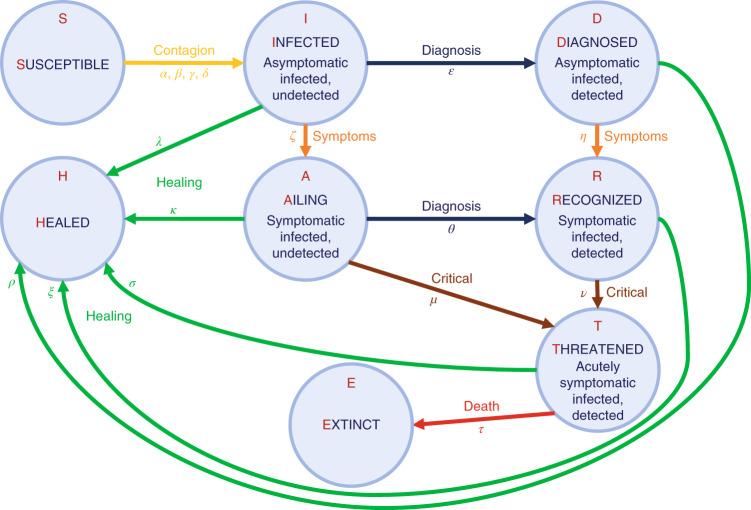
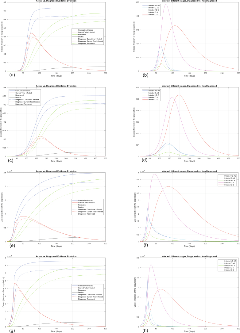
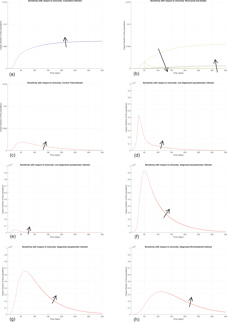
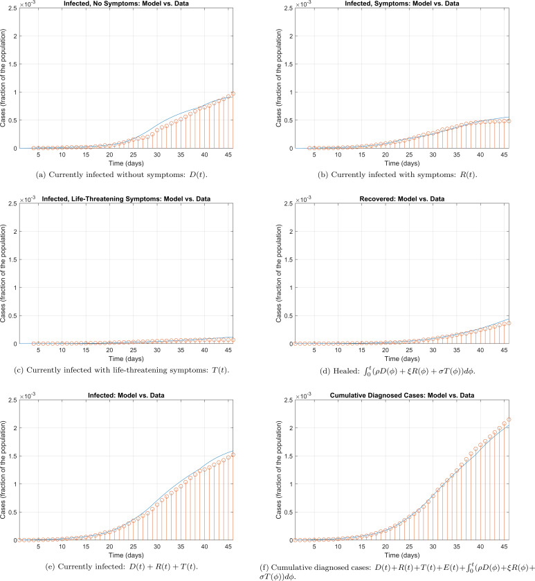
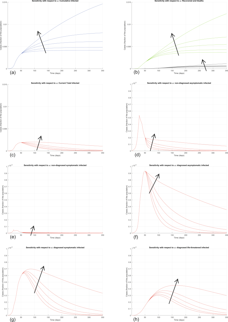
In Italy, 128,948 confirmed cases and 15,887 deaths of people who tested positive for SARS-CoV-2 were registered as of 5 April 2020. Ending the global SARS-CoV-2 pandemic requires implementation of multiple population-wide strategies, including social distancing, testing and contact tracing. We propose a new model that predicts the course of the epidemic to help plan an effective control strategy. The model considers eight stages of infection: susceptible (S), infected (I), diagnosed (D), ailing (A), recognized (R), threatened (T), healed (H) and extinct (E), collectively termed SIDARTHE. Our SIDARTHE model discriminates between infected individuals depending on whether they have been diagnosed and on the severity of their symptoms. The distinction between diagnosed and non-diagnosed individuals is important because the former are typically isolated and hence less likely to spread the infection. This delineation also helps to explain misperceptions of the case fatality rate and of the epidemic spread. We compare simulation results with real data on the COVID-19 epidemic in Italy, and we model possible scenarios of implementation of countermeasures. Our results demonstrate that restrictive social-distancing measures will need to be combined with widespread testing and contact tracing to end the ongoing COVID-19 pandemic.

Fig. 1. The model.

Graphical scheme representing the interactions among different stages of infection in the mathematical model SIDARTHE: S, susceptible (uninfected); I, infected (asymptomatic or pauci-symptomatic infected, undetected); D, diagnosed (asymptomatic infected, detected); A, ailing (symptomatic infected, undetected); R, recognized (symptomatic infected, detected); T, threatened (infected with life-threatening symptoms, detected); H, healed (recovered); E, extinct (dead).

Fig. 2. Fitted and predicted epidemic evolution.

Epidemic evolution predicted by the model based on the available data about the COVID-19 outbreak in Italy. a,b, The short-term epidemic evolution obtained by reproducing the data trend with the model. c,d, The long-term predicted evolution over a 350-day horizon. a,c, The difference between the actual evolution of the epidemic (solid lines; this refers to all cases of infection, both diagnosed and non-diagnosed, predicted by the model, although non-diagnosed cases are of course not counted in the data) and the diagnosed epidemic evolution (dashed lines; this refers to all cases that have been diagnosed and are thus reported in the data). The plots in b and d distinguish between the different categories of infected patients: non-diagnosed asymptomatic (ND AS), diagnosed asymptomatic (D AS), non-diagnosed symptomatic (ND S), diagnosed symptomatic (D S) and diagnosed with life-threatening symptoms (D IC). Note that a,c and b,d have different scales.

Fig. 3. The effect of lockdown.

a–d, Epidemic evolution predicted by the model for the COVID-19 outbreak in Italy when, after day 50, the social distancing countermeasures are weakened, leading to a larger R₀ = 0.98 (a,b), or strengthened, leading to a smaller R₀ = 0.50 (c,d). a,c, The difference between the actual (real cases) and perceived (diagnosed cases) evolution of the epidemics. The plots in b and d distinguish between the different categories of infected patients: non-diagnosed asymptomatic (ND AS), diagnosed asymptomatic (D AS), non-diagnosed symptomatic (ND S), diagnosed symptomatic (D S) and diagnosed with life-threatening symptoms (D IC). Note that a,c and b,d have different scales.

Fig. 4. The effect of testing.

a–d, Epidemic evolution predicted by the model for the COVID-19 outbreak in Italy when, after day 50, massive testing and contact tracing is enforced (a,b), leading to R₀ = 0.59, as well as in parallel with weakening social-distancing measures (c,d), leading to R₀ = 0.77. The plots in a and c show the difference between the actual (real cases) and the perceived (diagnosed cases) evolution of the epidemics. The plots in b and d distinguish between the different categories of infected patients: non-diagnosed asymptomatic (ND AS), diagnosed asymptomatic (D AS), non-diagnosed symptomatic (ND S), diagnosed symptomatic (D S) and diagnosed with life-threatening symptoms (D IC). Note that a,c and b,d have different scales.

Extended Data Fig. 1. Alternative scenarios for epidemic evolution.

Epidemic evolution that would have been predicted by the model for the COVID-19 outbreak in Italy if, after day 22, social-distancing countermeasures had been: absent (panels a and b), mild (panels c and d), strong (panels e and f) and very strong (panels g and h). In all cases, the actual Case Fatality Rate is around 7.2%, while the perceived CFR is around 9.0%. Panels (a), (c), (e), (g) show the difference between the actual (real cases) and the perceived (diagnosed cases) evolution of the epidemics, while panels (b), (d), (f), (h) distinguish between the different categories of infected patients. Note the different scales between the panels, having different orders of magnitude, which testify the enormous impact of social-distancing and lockdown.

Extended Data Fig. 2. Sensitivity analysis with respect to loss of immunity.

Sensitivity analysis showing the effect of introducing lack of immunity (hence, the possibility of reinfection) after day 50: recovered individuals can become susceptible again, so we add a term +χH(t) in equation (1) and a term −χH(t) in equation (7), where χ represents the rate at which immunity is lost. We show the evolution of the various model variables when χ = 0, χ = 0.1, χ = 0.8. Panel (a) shows the variation in the total number of cases, panel (b) in the number of recovered individuals (green) and deaths (black), panel (c) in the total number of currently infected individuals, panels (d)–(h) in the number of infected in different categories. Apart from the number of recovered individuals, which is drastically reduced after loss of immunity, all the other curves are essentially unaffected: the increase in the number of infected and deaths, hence the increase in the number of cumulative infected, is hardly visible.

Extended Data Fig. 3. Model simulation compared to real data.

Comparison between the official data (red dots histogram) and the results with the calibrated SIDARTHE model (blue line). Panel (a): number of reported infected with no (or mild) symptoms, who are quarantined at home. Panel (b): number of reported infected with symptoms, who are hospitalised. Panel (c): number of reported infected with life-threatening symptoms, admitted to ICU. Panel (d): number of reported recovered individuals. Panel (e): total number of reported infected in all categories. Panel (f): number of cumulative reported cases.

Extended Data Fig. 4. Sensitivity analysis with respect to α.

Sensitivity analysis showing the effect of varying the transmission coefficient α, whose nominal value is α = 0.21, after day 50. We multiply the nominal value of α by 0.5, 0.8, 1, 1.1, and 1.2, and show the corresponding evolution of the model variables. Panel (a) shows the variation in the total number of cases, panel (b) in the number of recovered individuals (green) and deaths (black), panel (c) in the total number of currently infected individuals, panels (d)–(h) in the number of infected in different categories. Increasing α significantly increases all the curves: the model is extremely sensitive to variations in the value of α.

Extended Data Fig. 5. Sensitivity analysis with respect to β.

Sensitivity analysis showing the effect of varying the transmission coefficient β, whose nominal value is β = 0.0050, after day 50. We multiply the nominal value of β by 0.5, 0.8, 1, 1.2, 2, and show the corresponding evolution of the model variables. Panel (a) shows the variation in the total number of cases, panel (b) in the number of recovered individuals (green) and deaths (black), panel (c) in the total number of currently infected individuals, panels (d)–(h) in the number of infected in different categories. Increasing β increases all the curves, although the sensitivity is smaller than with respect to α.

Extended Data Fig. 6. Sensitivity analysis with respect to γ.

Sensitivity analysis showing the effect of varying the transmission coefficient γ, whose nominal value is γ = 0.11, after day 50. We multiply the nominal value of γ by 0.5, 0.8, 1, 1.2, 2, and show the corresponding evolution of the model variables. Panel (a) shows the variation in the total number of cases, panel (b) in the number of recovered individuals (green) and deaths (black), panel (c) in the total number of currently infected individuals, panels (d)–(h) in the number of infected in different categories. Increasing γ increases all the curves, although the sensitivity is smaller than with respect to α and β.

Extended Data Fig. 7. Sensitivity analysis with respect to δ.

Sensitivity analysis showing the effect of varying the transmission coefficient δ, whose nominal value is δ = 0.0050, after day 50. We multiply the nominal value of δ by 0.5, 0.8, 1, 1.2, 2, and show the corresponding evolution of the model variables. Panel (a) shows the variation in the total number of cases, panel (b) in the number of recovered individuals (green) and deaths (black), panel (c) in the total number of currently infected individuals, panels (d)–(h) in the number of infected in different categories. Increasing δ increases all the curves, although the sensitivity is smaller than with respect to α.

Extended Data Fig. 8. Sensitivity analysis with respect to ε.

Sensitivity analysis showing the effect of varying the testing coefficient ε, whose nominal value is ε = 0.2000, after day 50. We multiply the nominal value of ε by 0.75, 0.8, 1, 1.2, 2, and show the corresponding evolution of the model variables. Panel (a) shows the variation in the total number of cases, panel (b) in the number of recovered individuals (green) and deaths (black), panel (c) in the total number of currently infected individuals, panels (d)–(h) in the number of infected in different categories. Increasing ε significantly decreases all the curves: the model is extremely sensitive to variations in the value of ε.

Extended Data Fig. 9. Sensitivity analysis with respect to θ.

Sensitivity analysis showing the effect of varying the testing coefficient θ, whose nominal value is θ = 0.3705, after day 50. We multiply the nominal value of θ by 0.5, 0.8, 1, 1.2, 2, and show the corresponding evolution of the model variables. Panel (a) shows the variation in the total number of cases, panel (b) in the number of recovered individuals (green) and deaths (black), panel (c) in the total number of currently infected individuals, panels (d)–(h) in the number of infected in different categories. Increasing θ decreases all the curves, but the sensitivity is smaller than with respect to ε.

Extended Data Fig. 10. Sensitivity analysis with respect to the other parameters.

Sensitivity analysis showing the effect of varying, after day 50: the worsening coefficients ζ and η leading to clinically relevant symptoms, whose nominal values are ζ = η = 0.0250 (row a); the worsening coefficients μ and ν leading to life-threatening symptoms, whose nominal values are μ = 0.0080 and ν = 0.0150 (row b); the healing coefficient λ, whose nominal value is λ = 0.0800 (row c); the healing coefficients ρ, κ, ξ and σ, whose nominal values are ρ = κ = ξ = 0.0200 and σ = 0.0100 (row d); the mortality coefficient τ, whose nominal value is τ = 0.0100 (row e). In all cases, the nominal value of all the considered parameters is multiplied by 0.5, 0.8, 1, 1.2, 2, and the corresponding evolution of the model variables is shown. Increasing ζ and η decreases the final number of infected and recovered, but also increases the number of deaths; the number of symptomatic and life-threatening infections initially increases, to decrease afterwards. Increasing μ and ν decreases the final number of infected and recovered, but also increases the number of deaths; the number of life-threatening infections initially increases, to decrease afterwards. Increasing λ, as well as the other healing parameters, decreases all the curves, apart from the curve of recovered patients, which initially increases (due to a higher recovery rate) and then eventually decreases (due to less infections overall). Increasing τ leaves all the curves almost unaffected, apart from the curve of life-threatened infected that is decreased, leading to a small decrease in the curve of all infected cases, the curve of recovered that is decreased and the curve of deaths that is increased.

References

1. Velavan TP, Meyer CG. The COVID-19 epidemic. Trop. Med. Int. Health. 2020;25:278–280. doi: 10.1111/tmi.13383. - DOI - PMC - PubMed
1. Wu Z, McGoogan JM. Characteristics of and important lessons from the coronavirus disease 2019 (COVID-19) outbreak in China: summary of a report of 72,314 cases from the Chinese center for disease control and prevention. JAMA. 2020;323:1239–1242. doi: 10.1001/jama.2020.2648. - DOI - PubMed
1. Guan, W.-J.et al. Clinical characteristics of coronavirus disease 2019 in China. N. Engl. J. Med.10.1056/NEJMoa2002032 (2020). - PMC - PubMed
1. WHO. Coronavirus Disease 2019 (COVID-19): Situation Report 76 (WHO, 2020).
1. Remuzzi A, Remuzzi G. COVID-19 and Italy: what next? Lancet Health Policy. 2020;395:1225–1228. - PMC - PubMed
Publication types