Dimensionality, information and learning in prefrontal cortex

Abstract

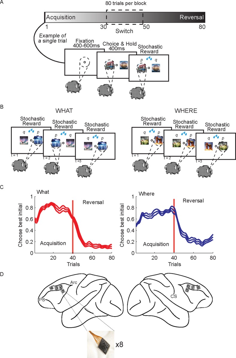
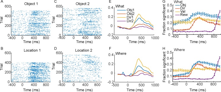
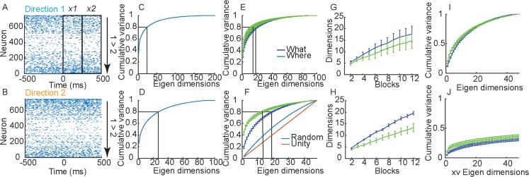
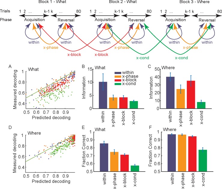
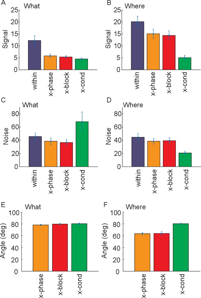
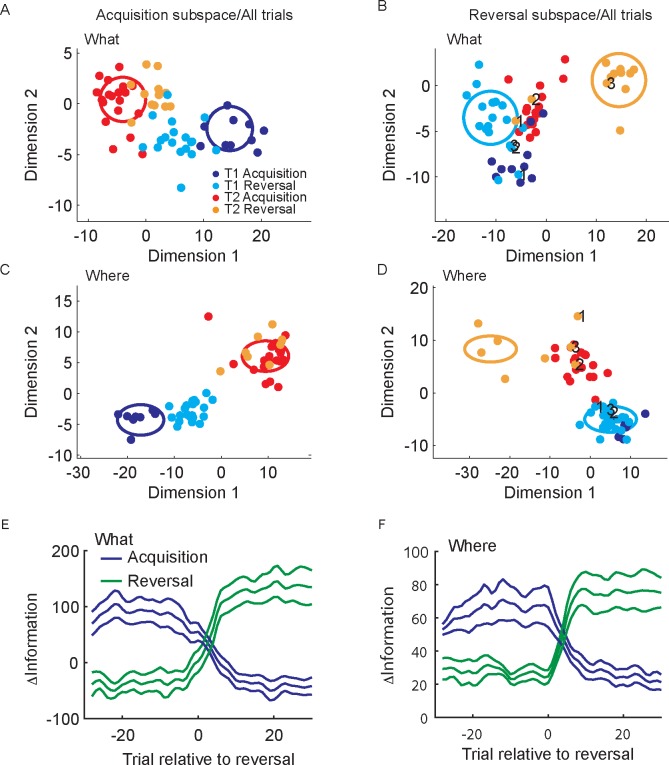
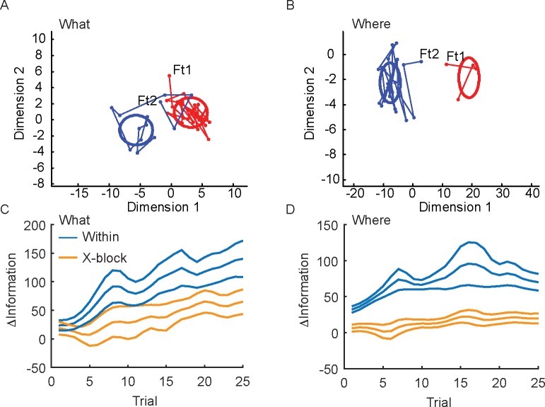
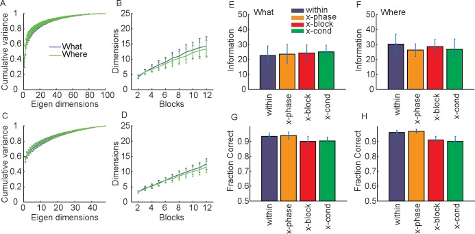
Learning leads to changes in population patterns of neural activity. In this study we wanted to examine how these changes in patterns of activity affect the dimensionality of neural responses and information about choices. We addressed these questions by carrying out high channel count recordings in dorsal-lateral prefrontal cortex (dlPFC; 768 electrodes) while monkeys performed a two-armed bandit reinforcement learning task. The high channel count recordings allowed us to study population coding while monkeys learned choices between actions or objects. We found that the dimensionality of neural population activity was higher across blocks in which animals learned the values of novel pairs of objects, than across blocks in which they learned the values of actions. The increase in dimensionality with learning in object blocks was related to less shared information across blocks, and therefore patterns of neural activity that were less similar, when compared to learning in action blocks. Furthermore, these differences emerged with learning, and were not a simple function of the choice of a visual image or action. Therefore, learning the values of novel objects increases the dimensionality of neural representations in dlPFC.

Fig 1. Two-armed bandit reinforcement learning task, behavior and recording locations.

A. The task was carried out in 80 trial blocks. At the beginning of each block of trials, 2 new images were introduced that the animal had not seen before. In each trial the animals fixated, and then two images were presented. The images were randomly presented left and right of fixation. Monkeys made a saccade to indicate their choice and then they were stochastically rewarded. B. There were two conditions. In the What condition one of the images was more frequently rewarded (p = 0.7) independent of which side it appeared on, and one of the images was less frequently rewarded (p = 0.3). In the Where condition one of the saccade directions was more frequently rewarded (p = 0.7) and one was less frequently rewarded (p = 0.3) independent of which image was at the chosen location. The condition remained fixed for the entire block. However, on a randomly chosen trial between 30 and 50, the reward mapping was reversed and the less frequently chosen object or location became more frequently rewarded, and vis-versa. C. Choice behavior across sessions. Animals quickly learned the more frequently rewarded image (left panel) or direction (right panel), and reversed their preferences when the choice-outcome mapping reversed. Because the number of trials in the acquisition and reversal phase differed across blocks, the trials were interpolated in each block to make all phases of equal length before averaging. The choice data was also smoothed using Gaussian kernel regression (kernel width sd = 1 trial). Thin lines indicate s.e.m. across sessions (n = 6 of each condition). D. Schematic shows locations of recording arrays, 4 in each hemisphere. Array locations were highly similar across animals.

Fig 2. Single cell example and single cell population statistics.

Time 0 is cue onset. Rasters and spike density functions for the example neuron are in panels A-F. A. Responses to choosing Object 1 in the What condition. B. Responses to direction/location 1 in the Where condition. C. Responses to choosing Object 2 in the What condition. D. Responses to choosing direction/location 2 in the Where condition. E. Average responses for the single neuron shown in A-D in the What condition. Average of the spike density functions for the preferred (Obj 1) vs. non-preferred (Obj 2) objects, or direction 1 or 2. F. Same as E for the Where condition. G. Fraction of neurons across the population significant in an ANOVA for each factor indicated, in the What condition. H. Same as G for the Where condition. Solid lines are averages across sessions (N = 6, 3 from each animal) and error bars are s.e.m. across sessions.

Fig 3. Single trial representations.

A. Raster showing the response of a population of simultaneously recorded neurons from a single trial when the animal chose Direction 1 in a trial from the Where condition. Outline boxes show time windows, x₁ and x₂, used to define activity vectors in analyses. B. Same as A for choice of Direction 2. C. Cumulative fraction of variance explained in trial-averaged responses (i.e. the vectors μ_i from each block and phase) across all blocks of both conditions. Note that the matrix only has 192 independent dimensions, so the cumulative variance saturates at 1 in dimension 192. D. Same as C for information dimensions, w = μ₂ − μ₁. This matrix has 96 dimensions, so cumulative variance saturates in dimension 96. E. Cumulative fraction of variance explained in trial-averaged responses (i.e. the vectors μ_i from each block and phase). Data is split out by What (Blue) and Where (Green) blocks. F. Same as E for informative dimensions, w. In addition, we also plot the dimensionality of a matrix with the same dimensionality, but with vectors chosen to have random directions, and also the unity line which has a constant increase in variance. G. Dimensionality of trial averaged responses as a function of number of blocks included in analysis. As we accumulate blocks in the analysis the dimensionality increases, also showing that the means do not all lie in the same subspace. The y-axis was estimated by calculating the number of dimensions required to account for 80% of the variance in the PSTHs as we aggregated randomly selected blocks. Note that the more independent (orthogonal) are the PSTHs in different blocks, the more dimensions will be required to span them as we aggregate across blocks. H. Same as G for the informative dimensions. I. Cumulative variance accounted for in informative dimensions, w, after removing the first principal component from both What and Where conditions. J. Cumulative variance accounted for with cross validation.

Fig 4. Information in subspace defined in various ways.

Error bars in bar plots are s.e.m. and n = 6 (i.e. sessions) in all cases. Diagram at the top shows example of how comparisons are defined. A. Relation between predicted and measured decoding performance for What condition. Units are fraction correct. B. Information in the What condition in subspaces defined for the current block and phase (within), for the opposite phase from the same block (x-phase), for the same phase for other blocks of the same type (x-block) and for the same phase for other blocks of the other type (x-cond). C. Same as B for the Where condition. D. Relation between predicted and measured decoding performance for Where condition. Units are fraction correct. E. Decoding performance shown as fraction correct for the What condition. F. Same as E for the Where condition.

Fig 5. Signal, noise and principal angle.

A. Signal (which for linear information is the norm of the difference in the mean responses in the two conditions, i.e. the norm of w = μ₂−μ₁) for the What condition, after projecting data into each subspace. The subspace for a single block is given by activity in the two time bins (i.e. 0–250 ms after cue onset and 251–500 ms after cue onset). B. Same as A for the Where condition. C Noise (Trace of the noise covariance matrix, after projecting data into corresponding subspace) for the What condition. D. Same as C for the Where condition. E. Principal angles for the What condition. This is the angle between the subspace for the current block and the opposite phase of the current block (x-phase), other blocks of the same type (x-block) and other blocks of the other type (x-cond). Note the principal angle is given by the matrix norm of the matrix of dot products between all dimensions of each subspace. F. Principal angles for the Where condition. The principal angle is larger between subspaces for different blocks of the What condition than the where condition.

Fig 6. Population activity in acquisition and reversal subspaces.

A. Projection of single trial population activity from the acquisition and reversal phases into subspace defined for the acquisition block for an example What block. Each dot is a trial. T1 is target 1 and T2 is target 2. Dimensions are rotations within the subspace spanned by the two time bins, from 0–250 and 251–500 ms after cue onset. The dimensions were found by computing the eigenvectors for the covariance across these two time bins. B. Projection of single trial population activity from both phases into the subspace identified for the reversal phase. Dot color indicates phase and object chosen. Numbers indicate trials after reversal: 1 is first trial after, 2 is second trial, etc. C. Same as A for an example Where block. D. Same as B for an example Where block. E. Average difference in distances in subspaces identified for acquisition and reversal for What blocks. F. Same as E for Where blocks. Error bars are s.e.m. N = 6.

Fig 7. Convergence of population activity with learning.

A. Example block of trials in which the population activity initially starts far from the distribution of activity after learning. Activity evolves and converges to the post-learning distribution. Ft1 is the first trial for object 1 and Ft2 is the first trial for object 2. Additional linked points are subsequent trials of the same choice, which are not necessarily consecutive trials in the task. Because the number of times each option was chosen in each block varies, the number of points varies. Option 1 was chosen more often than option 2 in this example block. Ellipses show 1 standard deviation of data for each condition. Dimensions 1 and 2 on the x and y axes refer to the subspace for each block, which is defined by rotations within the subspace spanned by the activity in the two time bins (i.e. 0–250 and 251–500 ms after cue onset). B. Same as A for an example Where block. C. Separation of population activity patterns with learning, in both the within and x-block subspaces for the What blocks. Y-axis indicates the difference between the Mahalanobis distances of the single trial activity to the mean for the opposite vs. same condition (see methods). Larger distances indicate further from the opposite choice distribution and closer to the correct choice distribution. D. Same as C for the Where blocks. Note, values for x-block ΔInformation are low because we did not re-estimate means after projection for this analysis, as we did for the analyses in Fig 4. Error bars are s.e.m. with n = 6.

Fig 8. Dimensionality and information in reward related activity.

A. Cumulative fraction of variance explained in trial-averaged responses to the reward (i.e. the vectors μ_i from each block and phase where μ₁ is the activity for reward and μ₂ is the activity for no reward) across all blocks split out by condition. B. Number of eigen dimensions necessary to account for 80% of the variance as a function of the number of blocks included in the analysis. C. Same as A for informative dimensions, w = μ₂−μ₁, where again μ₁ is the activity for reward and μ₂ is the activity for no reward. D. Same as B for informative dimensions. E. Information about reward delivery in the What condition. F. Information about reward delivery in the Where condition. G. Fraction correct for the What condition, where prediction is whether a reward was or was not delivered. H. Same as G for the Where condition.

References

1. Sejnowski TJ. Neural populations revealed. Nature. 1988;332(24):308. - PubMed
1. Cunningham JP, Yu BM. Dimensionality reduction for large-scale neural recordings. Nat Neurosci. 2014;17(11):1500–9. 10.1038/nn.3776 - DOI - PMC - PubMed
1. Ganguli S, Sompolinsky H. Compressed sensing, sparsity, and dimensionality in neuronal information processing and data analysis. Annu Rev Neurosci. 2012;35:485–508. 10.1146/annurev-neuro-062111-150410 . - DOI - PubMed
1. Churchland MM, Cunningham JP, Kaufman MT, Foster JD, Nuyujukian P, Ryu SI, et al. Neural population dynamics during reaching. Nature. 2012;487(7405):51–6. 10.1038/nature11129 - DOI - PMC - PubMed
1. Williamson RC, Cowley BR, Litwin-Kumar A, Doiron B, Kohn A, Smith MA, et al. Scaling Properties of Dimensionality Reduction for Neural Populations and Network Models. PLoS Comput Biol. 2016;12(12):e1005141 10.1371/journal.pcbi.1005141 - DOI - PMC - PubMed
Publication types