Cryogenic Correlative Single-Particle Photoluminescence Spectroscopy and Electron Tomography for Investigation of Nanomaterials

Abstract

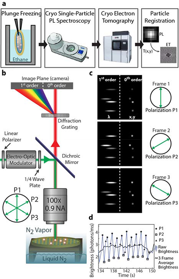
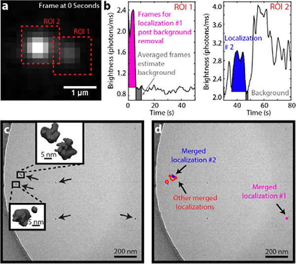
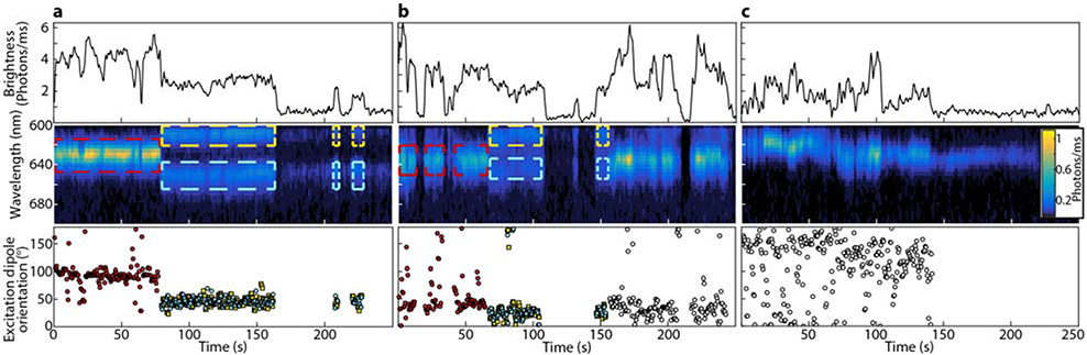
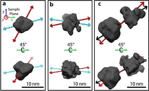
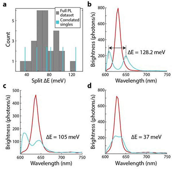
Cryogenic single-particle photoluminescence (PL) spectroscopy has been used with great success to directly observe the heterogeneous photophysical states present in a population of luminescent particles. Cryogenic electron tomography provides complementary nanometer scale structural information to PL spectroscopy, but the two techniques have not been correlated due to technical challenges. Here, we present a method for correlating single-particle information from these two powerful microscopy modalities. We simultaneously observe PL brightness, emission spectrum, and in-plane excitation dipole orientation of CdSSe/ZnS quantum dots suspended in vitreous ice. Stable and fluctuating emitters were observed, as well as a surprising splitting of the PL spectrum into two bands with an average energy separation of 80 meV. In some cases, the onset of the splitting corresponded to changes in the in-plane excitation dipole orientation. These dynamics were assigned to structures of individual quantum dots and the excitation dipoles were visualized in the context of structural features.

Keywords: correlative light electron microscopy (CLEM); cryogenic electron tomography; fluorescence spectroscopy; nanoparticles; single-molecule studies.

Figure 1.

Overview of experiment. (a) Outline of experimental workflow. Samples are plunge frozen to suspend QDs in vitreous ice, then fluorescently imaged. Cryo-ET is then conducted at 77K on the same sample, and the images are registered. (b) Schematic of home-built cryogenic widefield fluorescence microscope. The excitation laser is passed through a linear polarizer, an electro-optic modulator (EOM) and a quarter wave plate to produce excitation polarization modulated every frame (500 ms) in ~60° steps. Emission is dispersed onto an EMCCD camera by a diffraction grating. (c) Illustration of separation of position and spectral information on the EMCCD and change in brightness with changing excitation polarization. Different emitters show different response to excitation polarization based on their preferred in-plane excitation dipole orientation. (d) Example brightness trace for a single QD. In blue is the raw trace showing the three-frame periodic change in brightness due to the stepped excitation polarization. Frames at polarizations P1, P2, and P3 are marked with circles, empty squares, and triangles respectively. A three-frame moving average brightness is plotted in black to more clearly show changes in brightness not associated with changes in excitation polarization.

Figure 2.

Overlay of single-QD emission localizations and electron microscopy data. (a) Cropped region of a frame showing the 0^th order spots generated by two spatially separated emitters. (b) Intensity of the integrated areas shown as dashed red boxes in (a) as a function of time. In the rare cases where there is substantial overlap of the point spread functions from several emitters, as is the case for ROI 2, the contributions from individual emitters can be isolated by subtracting the average of frames adjacent in time to large intensity changes from blinking. The large signals (magenta and blue) above the estimated background (gray) can then be attributed to an individual emitter. (c) Medium magnification electron micrograph corresponding to the area shown in (a). Black arrows highlight the location of quantum dots. Inset shows the three-dimensional reconstruction from higher magnification cryo-ET. (d) Overlay of merged localizations shown as red circles. Magenta and blue circles correspond to the localizations from (b). The radius of the circles is the localization precision estimated by the standard error of the mean of the individual frame localizations.

Figure 3.

PL data for single QDs. For (a), (b) and (c), the top panel shows a three frame running average of the brightness extracted from the 0^th order image scaled by 5.8 to represent photons collected in both the 0^th and 1^st order images. The middle panels show a waterfall plot of the spectra extracted from the 1^st order image over time, also averaged over three frames. The smoothing is done to show changes in brightness not associated with changes in the excitation polarization. The bottom panel shows the in-plane excitation dipole orientation calculated for each frame from the current brightness and the brightness of the next two frames. Red circles, blue circles, and yellow squares show orientation calculated from brightness extracted from the spectral regions boxed in red, blue, and yellow respectively. Orientations marked with white circles are calculated from the brightness in the 0^th order spot over three consecutive frames.

Figure 4.

Correlation of PL orientation measurements and cryo-ET reconstructions. The upper images are a top down view, and the lower images are rotated 45° around horizontal. (a) Overlay of cryo-ET reconstructions (gray) and the excitation dipoles (red and cyan arrows) corresponding to the red and cyan boxes from Figure 3a. (b) Same as (a) except arrows and structure correspond to fluorescence data from Figure 3b. (c) A pair of dots that was observed to have a weak preference for excitation along the red arrow which aligns closely with the black line joining the centers of mass in xy plane.

Figure 5.

(a) Histogram of observed splitting energies in meV. Splitting energy is defined as the average energy difference between the center of two Gaussian functions fit to the split emission spectra. In cyan are the average splitting energies of each of the seven single QDs with correlated three-dimensional structure that exhibited split emission spectra. In grey are the average splitting energies of all objects that exhibited split emission spectra regardless of correlative data. (b-d) Time averaged spectrum from boxed time windows of the split and single-peaked state for the QD in (b) Figure 3a and 4b (c) 3b and 4b (d) Figure S5b.

References

-
- Murray CB, Kagan CR, Bawendi MG, Annu. Rev. Mater. Sci 2000, 30, 545–610.
- Moerner WE, Kador L, Phys. Rev. Lett 1989, 62, 2535–2538. - PubMed
- Personov RI, Al’Shits EI, Bykovskaya LA, Opt. Commun 1972, 6, 169–173.
- Empedocles S, Bawendi M, Acc. Chem. Res 1999, 32, 389–396.
- Naumov AV, Physics-Uspekhi 2013, 56, 605–622.
Publication types
MeSH terms
Substances
Grants and funding
LinkOut - more resources
Full Text Sources