Predicting ecosystem state changes in shallow lakes using an aquatic ecosystem model: Lake Hinge, Denmark, an example

Abstract

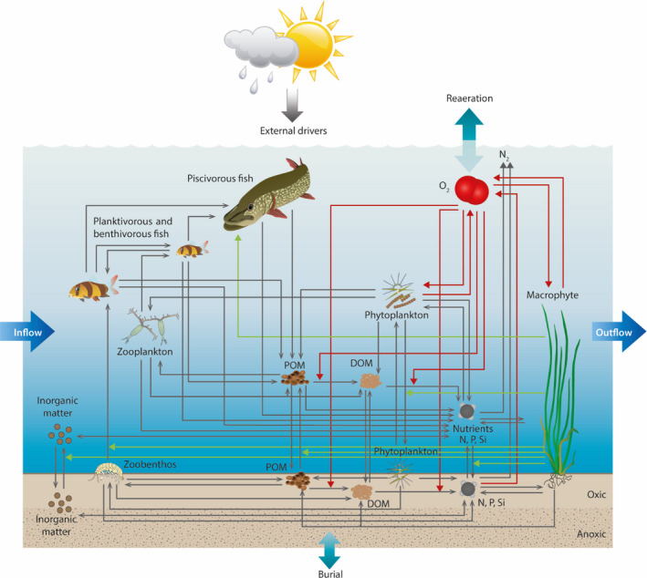
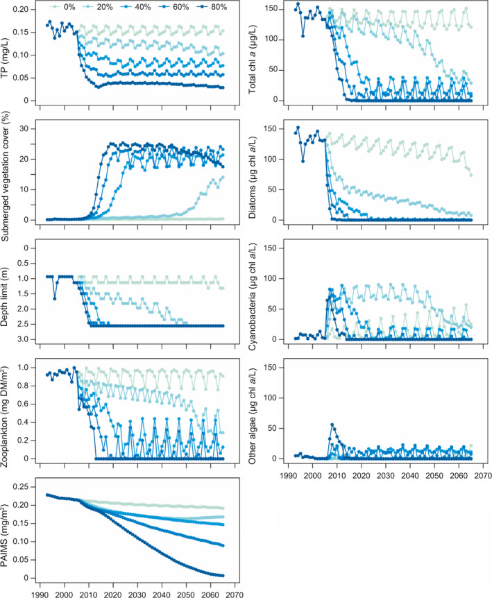
In recent years, considerable efforts have been made to restore turbid, phytoplankton-dominated shallow lakes to a clear-water state with high coverage of submerged macrophytes. Various dynamic lake models with simplified physical representations of vertical gradients, such as PCLake, have been used to predict external nutrient load thresholds for such nonlinear regime shifts. However, recent observational studies have questioned the concept of regime shifts by emphasizing that gradual changes are more common than sudden shifts. We investigated if regime shifts would be more gradual if the models account for depth-dependent heterogeneity of the system by including the possibility of vertical gradients in the water column and sediment layers for the entire depth. Hence, bifurcation analysis was undertaken using the 1D hydrodynamic model GOTM, accounting for vertical gradients, coupled to the aquatic ecosystem model PCLake, which is implemented in the framework for aquatic biogeochemical modeling (FABM). First, the model was calibrated and validated against a comprehensive data set covering two consecutive 7-yr periods from Lake Hinge, a shallow, eutrophic Danish lake. The autocalibration program Auto-Calibration Python (ACPy) was applied to achieve a more comprehensive adjustment of model parameters. The model simulations showed excellent agreement with observed data for water temperature, total nitrogen, and nitrate and good agreement for ammonium, total phosphorus, phosphate, and chlorophyll a concentrations. Zooplankton and macrophyte coverage were adequately simulated for the purpose of this study, and in general the GOTM-FABM-PCLake model simulations performed well compared with other model studies. In contrast to previous model studies ignoring depth heterogeneity, our bifurcation analysis revealed that the spatial extent and depth limitation of macrophytes as well as phytoplankton chlorophyll-a responded more gradually over time to a reduction in the external phosphorus load, albeit some hysteresis effects still appeared. In a management perspective, our study emphasizes the need to include depth heterogeneity in the model structure to more correctly determine at which external nutrient load a given lake changes ecosystem state to a clear-water condition.

Keywords: FABM-PCLake; General Ocean Turbulence Model; aquatic ecosystem modeling; critical nutrient loads; lake restoration; predictive ecology; regime shifts; shallow lakes; water quality.

Fig. 1

Study area covering the catchment of Lake Hinge, Denmark. Monitoring stations 1, 2, and 3 cover inlet streams from gauged catchment areas (shaded), station 4 represents the lake outlet and station 5 the in‐lake water quality sampling station. Land use classifications are derived from Nielsen et al. (2000).

Fig. 2

The relationship between lake level and surface area for Lake Hinge (thick black line) where level 0 m represents the deepest part of the lake. In the 1D GOTM‐FABM‐PCLake setup for Lake Hinge, the water column is composed of 16 water layers (gray lines) with a height between 10–21 cm and a sediment in each layer (illustrated by highlighted brown area). In comparison, the 0D PCLake setup for Lake Hinge (Janse et al. 2008) is a box model with one water layer (blue area) of 1.2 m (dashed line) with a connected sediment layer (illustrated by highlighted brown area).

Fig. 3

Conceptual figure of the aquatic ecosystem model FABM‐PCLake adapted from (Hu et al. 2016). Key state variables of FABM‐PCLake are shown and their interactions represented by gray arrows. Dissolved oxygen dynamics represented by red arrows and processes mediated by macrophytes are shown with green arrows.

Fig. 4

Conceptual depiction of the bifurcation analysis with 75 different external P load scenarios at two different initial ecosystem states, turbid and clear‐water (top and bottom plot, respectively) and their corresponding load‐response curve (gray center plot). A five‐year baseline from the validation period (2001–2006, orange band) was used to calculate new external phosphorus loadings in increments of 2% within a −98% to +50% range. Oligotrophication scenarios (top plot) were simulated with 12 repetitions of baseline (60 yr in total, light blue band) for all new external loadings, and summer means of the last five years of the simulation period (dark blue band) were extracted. Eutrophication scenarios (bottom plot) were simulated with a 98% P load reduction for 20 yr to establish a “clear‐water state” in the lake (light green band) following 12 repetitions of baseline (60 yr in total) (light green band) with all new external loading increases, and summer means of the last five years of the simulation period (dark green band) were extracted. Extracted summer means from both scenarios were then ranked and plotted according to their external mean P load in a load‐response curve (gray center plot). Baseline load in load‐response curve represents the 5‐yr external P load mean.

Fig. 5

Simulated model values (black lines) against observed values in the calibration and validation period (white circles and light gray band, black circles and dark gray band, respectively) for (a) temperature, (b) dissolved oxygen (DO), (c) total nitrogen (TN), and (d) total phosphorus (TP). TN and TP observations include 15% error band to indicate uncertainty related to observations.

Fig. 6

Simulated model values (black lines) against observed values in the calibration and validation period (white circles and light gray band, black circles and dark gray band, respectively) for (a) phosphate (PO₄), (b) nitrate (NO₃), (c) ammonium (NH₄), and (d) particulate organic matter (POM). All observations include a 15% error band to indicate uncertainty related to observations. DM, dry mass.

Fig. 7

Simulated model values for (a) chl a, (b) diatom, cyanobacteria, and other algae chl a, (c) macrophyte coverage, and (d) zooplankton biomass. (a) Simulated total chl a concentrations against observed values in calibration and validation period (light gray band and dark gray band, respectively). All observations include a 20% error band to indicate uncertainty related to observations. (b) Simulated phytoplankton chl a concentrations for each phytoplankton group (diatoms [orange], cyanobacteria [blue], and other algae [light blue]) with observed percentage of summer mean biovolume (mean and standard deviation) in inset. (c) Simulated macrophyte percent cover for depths 0.4 m (blue), 0.65 m (orange), 1.0 m (red), and 1.25 m (dark red) against observations (circles in corresponding color). (d) Simulated zooplankton biomass against observed values in the calibration and validation period (white circles and black circles, respectively).

Fig. 8

Load‐response curves from bifurcation analysis of summer means of the last 5 yr in an oligotrophication (green circles) and a eutrophication (blue circles) scenario for a −98% to + 50% change in external P load for various state variables. Dashed vertical line represents the calibrated state (no external P load change). Juv., juvenile; pl., zooplanktivorous; bt, zoobenthivorous; Pisc., piscivorous.

Fig. 9

Time series of summer means from five oligotrophication scenarios with an 80% to 0% P load reduction during the calibration (1993–2000), validation (2000–2007), and scenario (2005–2065, a looped 5‐yr period) periods for TP, macrophyte coverage and depth limit, chl a concentrations for total phytoplankton and individual phytoplankton groups, zooplankton biomass, and phosphorus bound to inorganic matter (PAIMS).

References

1. Aldenberg, T. , Janse J. H., and Kramer P. R. G.. 1995. Fitting the dynamic model PCLake to a multi‐lake survey through Bayesian Statistics. Ecological Modelling 78:83–99.
1. Arhonditsis, G. B. , Adams‐Vanharn B. A., Nielsen L., Stow C. A., and Reckhow K. H.. 2006. Evaluation of the current state of mechanistic aquatic biogeochemical modeling: Citation analysis and future perspectives. Environmental Science and Technology 40:6547–6554. - PubMed
1. Bennett, N. D. , et al. 2013. Characterising performance of environmental models. Environmental Modelling and Software 40:1–20.
1. Beven, K. 2006. A manifesto for the equifinality thesis. Journal of Hydrology 320:18–36.
1. Bjerring, R. , Windolf J., Kronvang B., Sørensen P. B., Timmermann A., Kjeldgaard A., Larsen S. E., Thodsen H., and Bøgestrand J.. 2014. Belastningsopgørelser til søer. Aarhus University, DCE – Danish Center for Energy and Environment, Silkeborg, Denmark.
Publication types
LinkOut - more resources