. 2020 May;17(5):531-540.
doi: 10.1038/s41592-020-0816-x. Epub 2020 May 4.

Three-dimensional nanoscopy of whole cells and tissues with in situ point spread function retrieval

Affiliations

Three-dimensional nanoscopy of whole cells and tissues with in situ point spread function retrieval

Fan Xu et al. Nat Methods. 2020 May.

Abstract

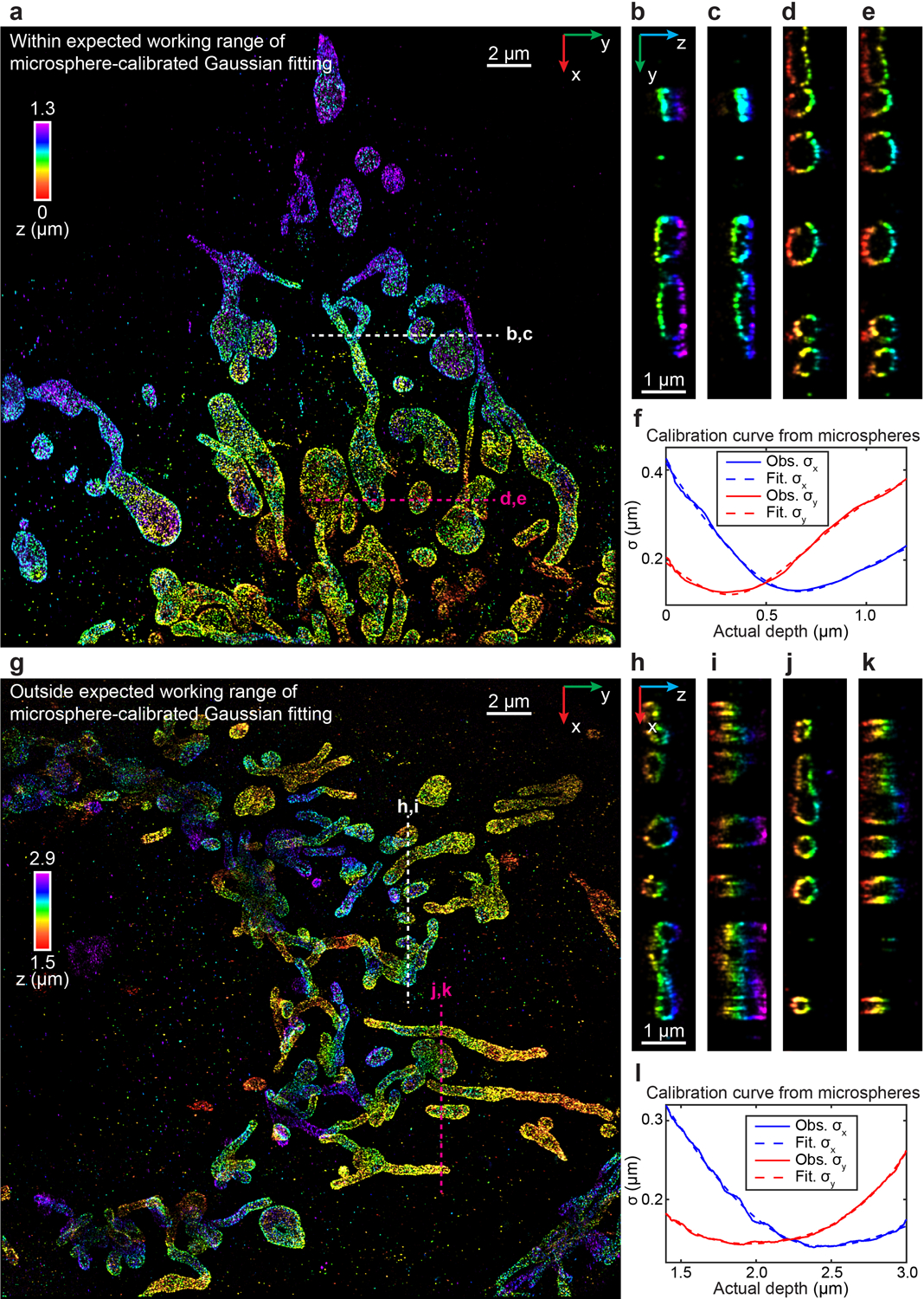
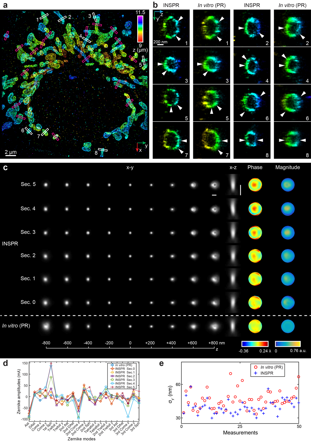
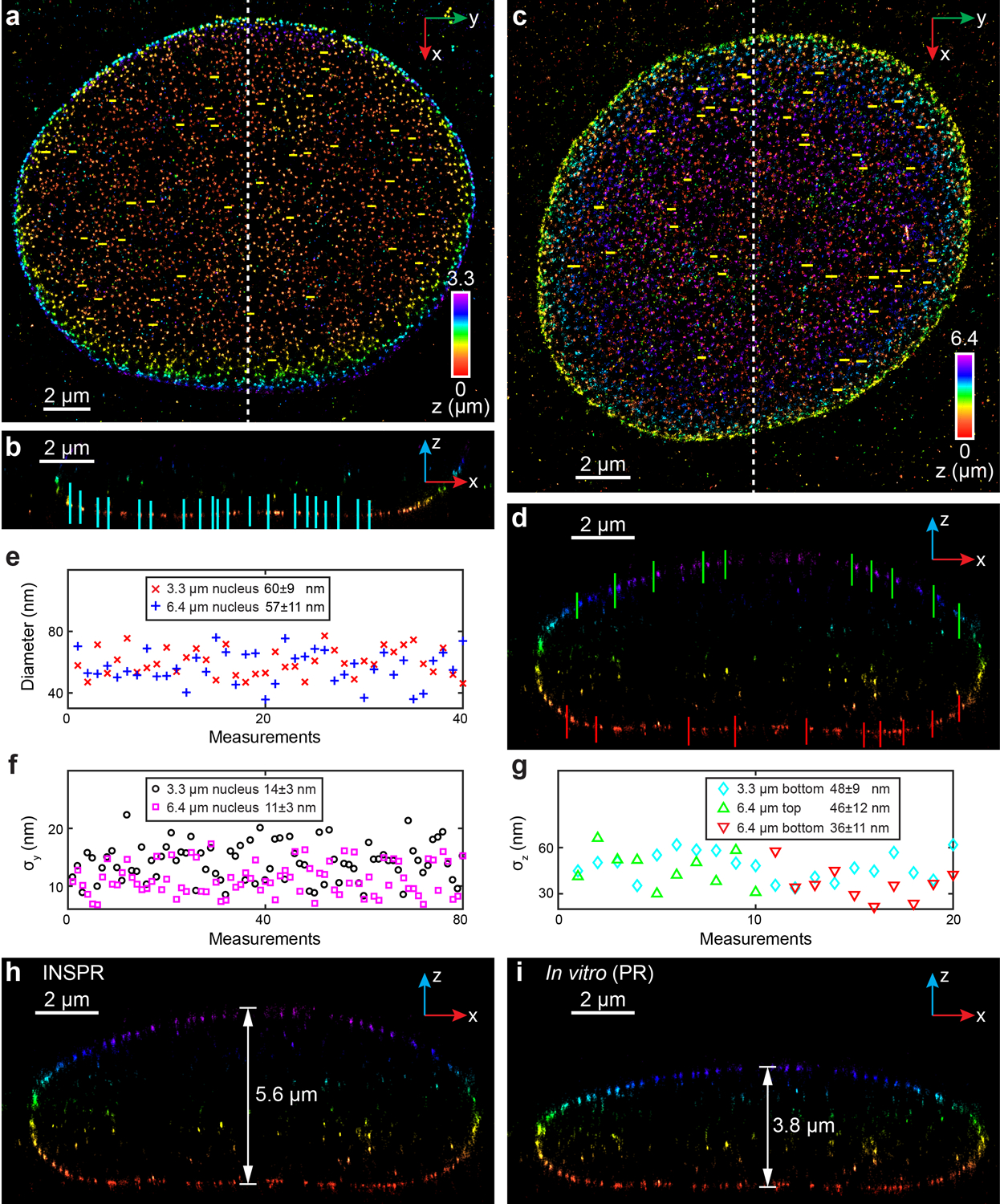
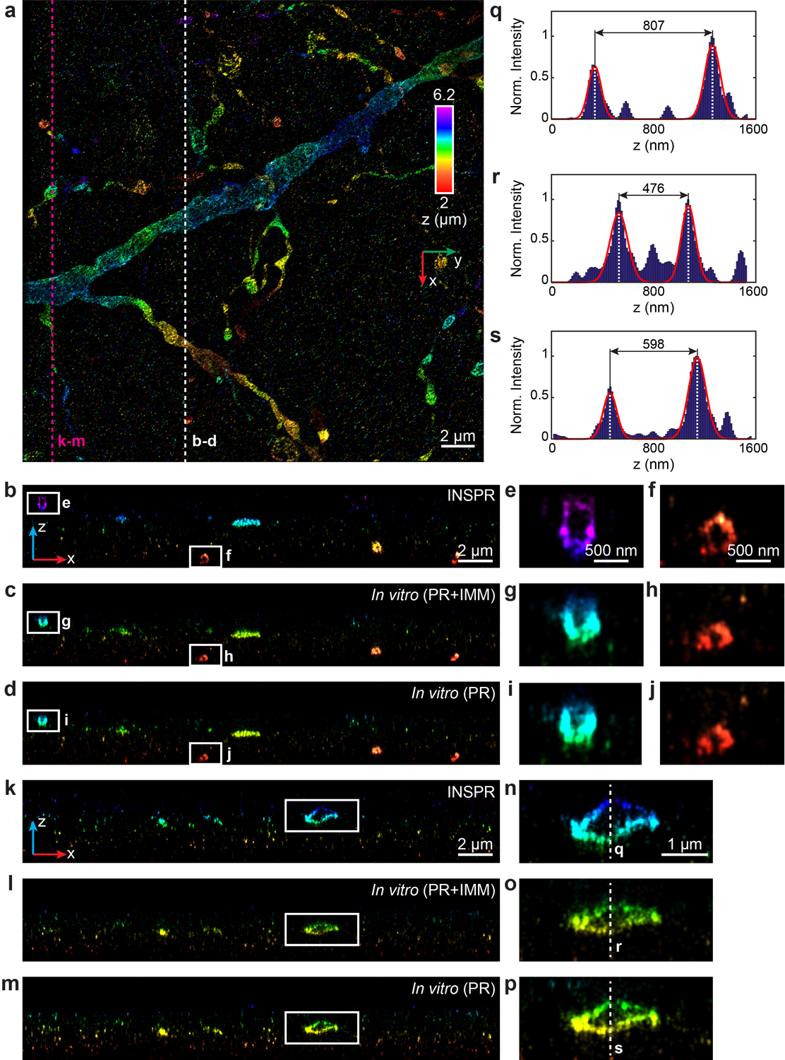
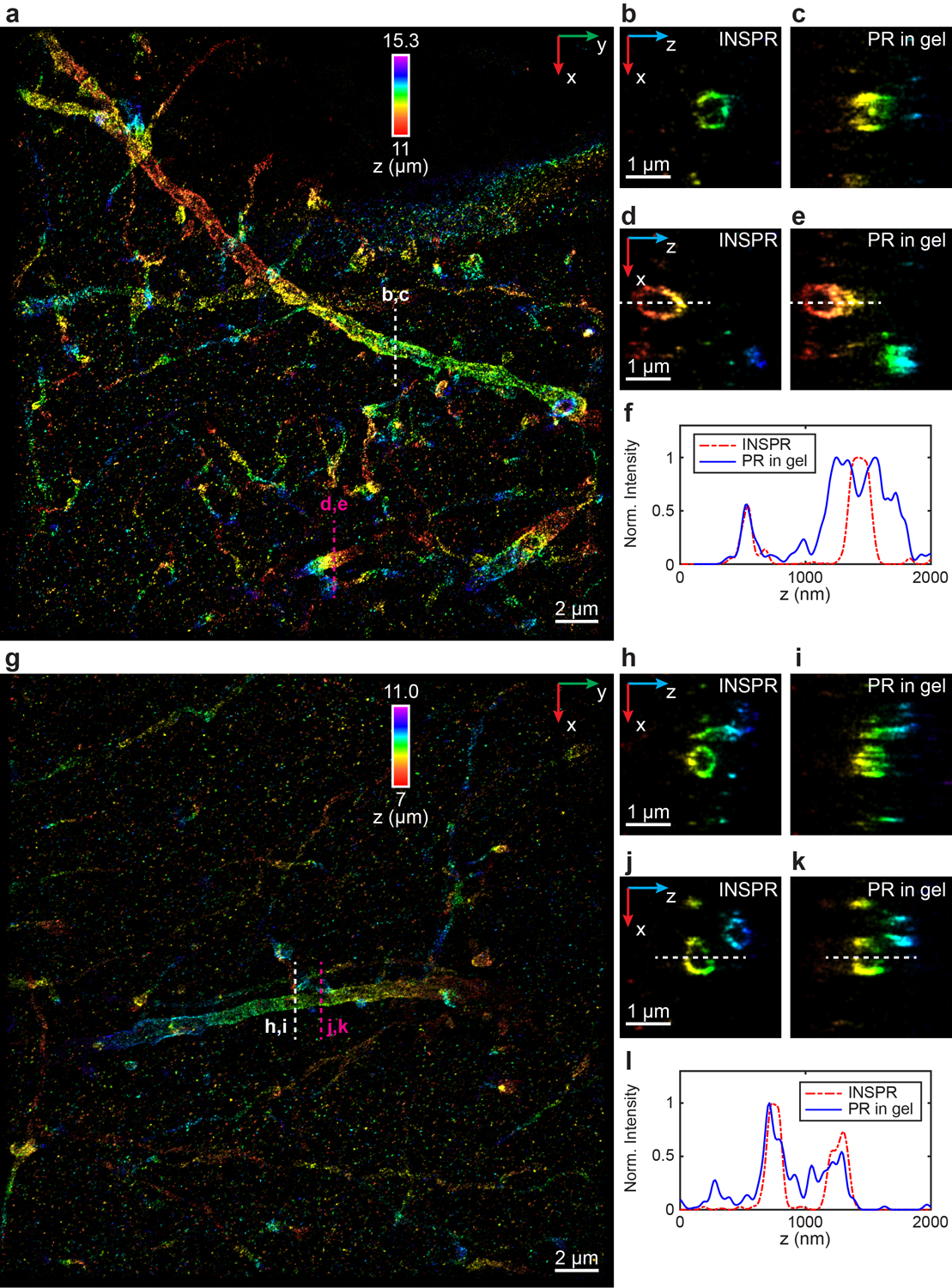
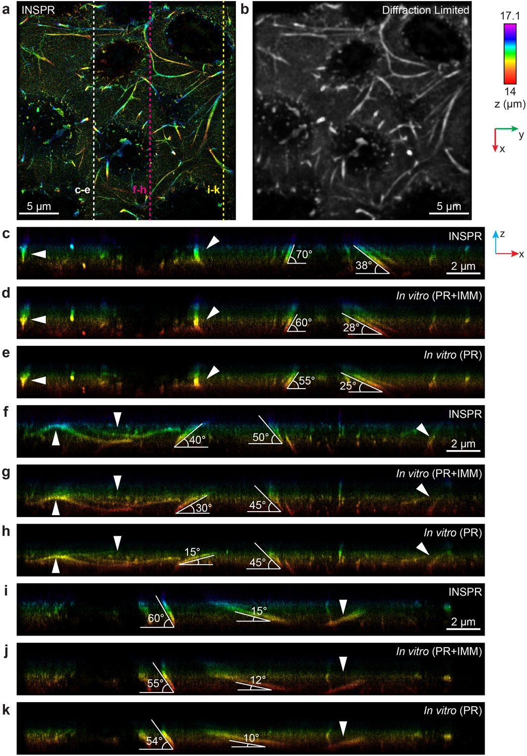
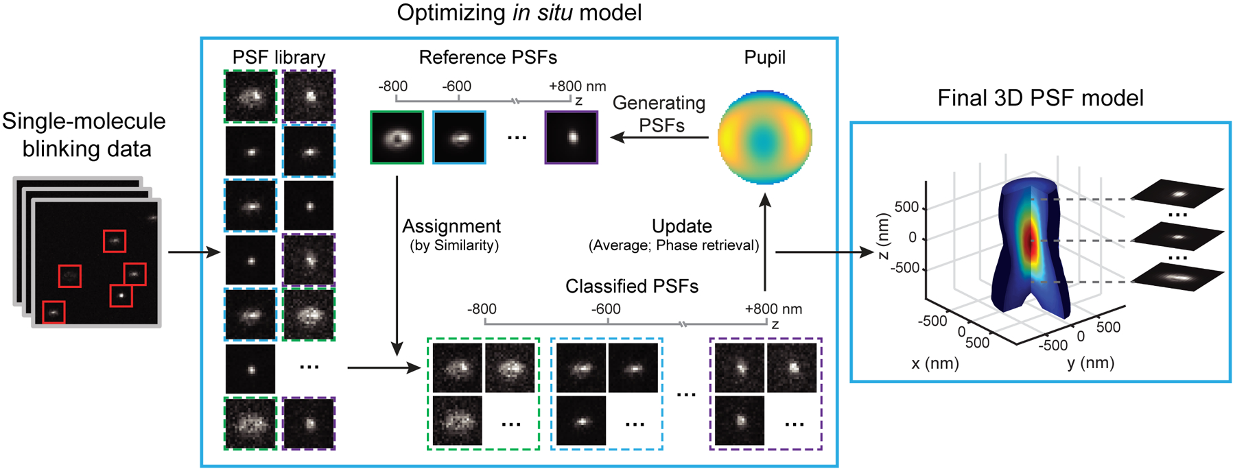
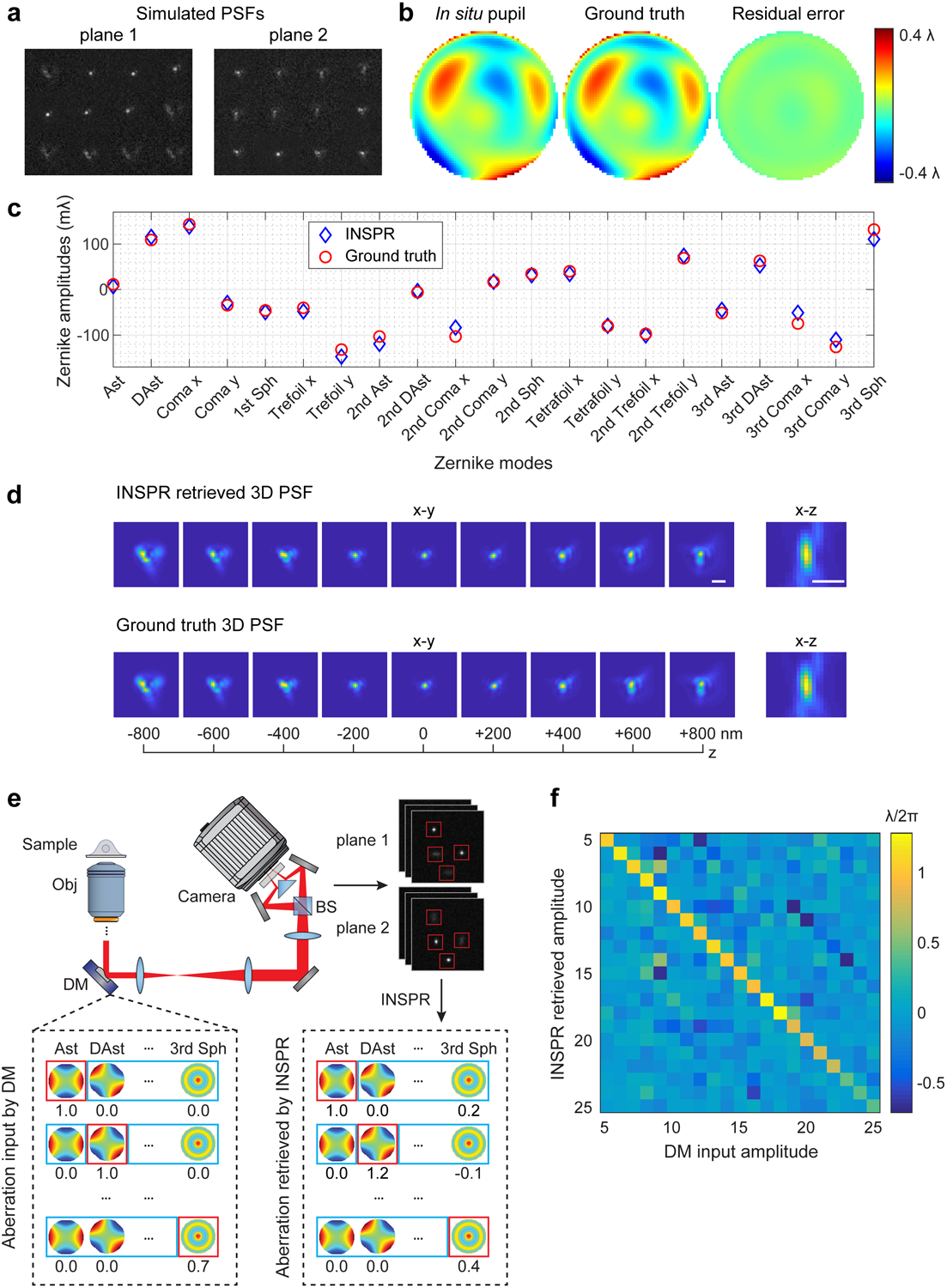
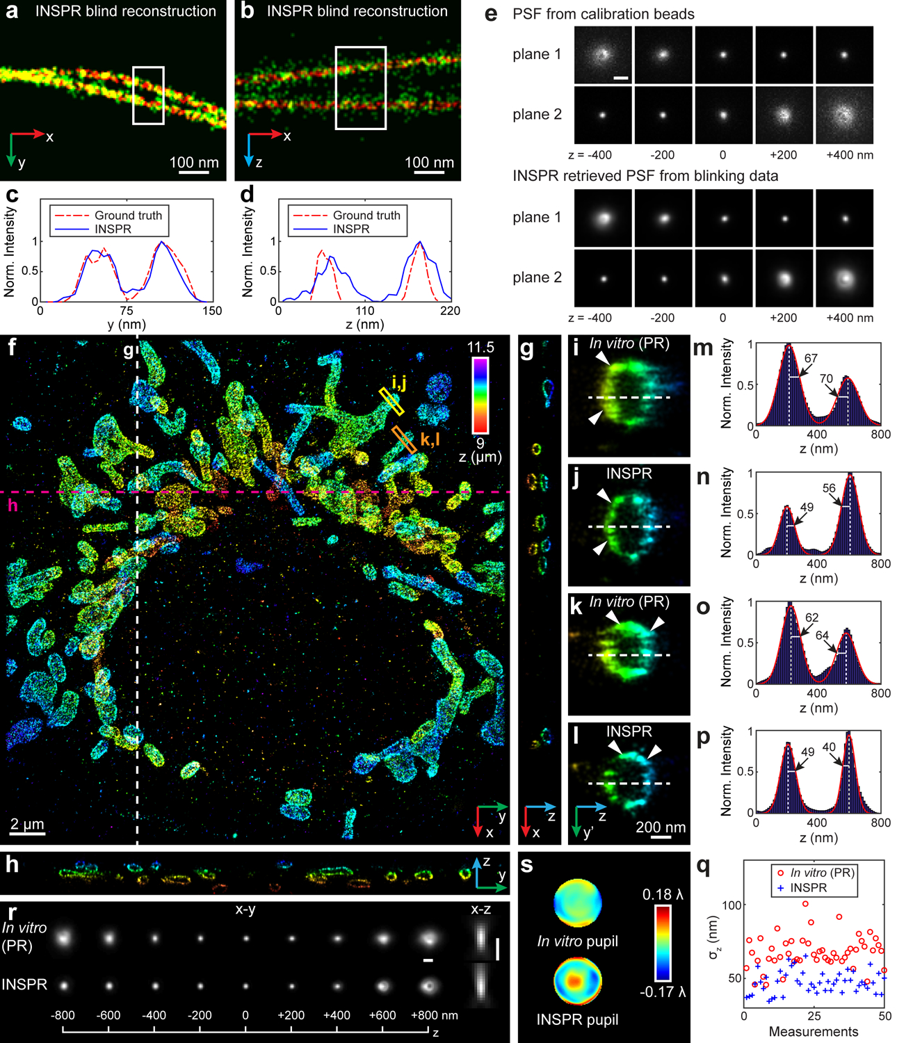
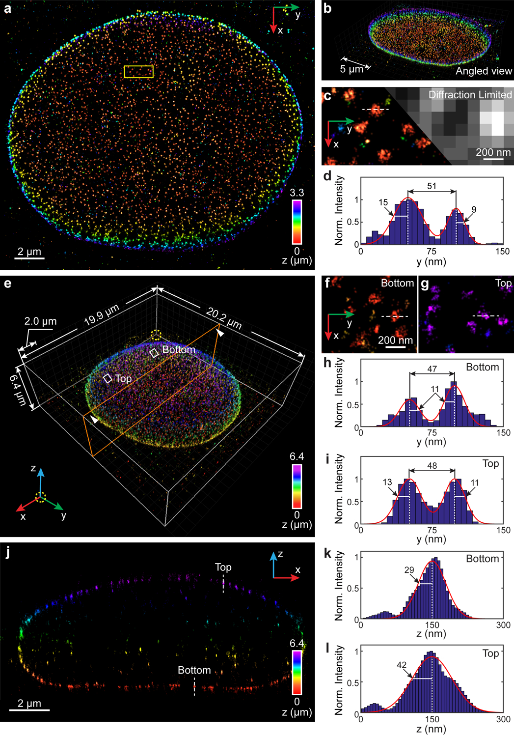
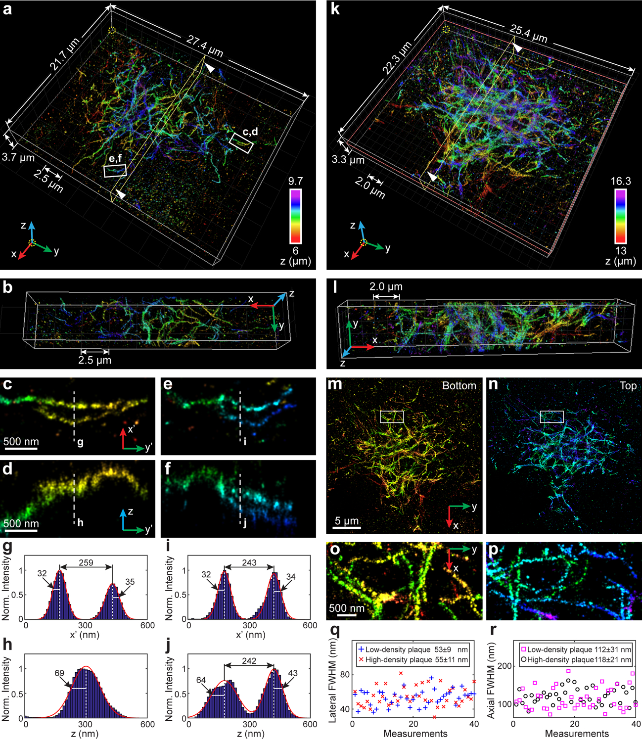
Single-molecule localization microscopy is a powerful tool for visualizing subcellular structures, interactions and protein functions in biological research. However, inhomogeneous refractive indices inside cells and tissues distort the fluorescent signal emitted from single-molecule probes, which rapidly degrades resolution with increasing depth. We propose a method that enables the construction of an in situ 3D response of single emitters directly from single-molecule blinking datasets, and therefore allows their locations to be pinpointed with precision that achieves the Cramér-Rao lower bound and uncompromised fidelity. We demonstrate this method, named in situ PSF retrieval (INSPR), across a range of cellular and tissue architectures, from mitochondrial networks and nuclear pores in mammalian cells to amyloid-β plaques and dendrites in brain tissues and elastic fibers in developing cartilage of mice. This advancement expands the routine applicability of super-resolution microscopy from selected cellular targets near coverslips to intra- and extracellular targets deep inside tissues.


Conflict of interest statement

Competing interests

F.X., D.M., and F.H. are inventors on patent application submitted by Purdue University that covers basic principles of INSPR.

Figures

Extended Data Fig. 1.
Extended Data Fig. 1.. INSPR framework, degeneracy illustration, and setup diagram.
(a) INSPR framework and detailed process of in situ model generation. (b) Single molecules are localized by a pair of channel-specific models which share the same shape information with the corresponding sub-regions. (c) Degeneracy exists in single plane configuration, where PSFs with positive and negative vertical astigmatism aberrations (Ast) are identical at opposite axial positions. (d) Degeneracy is broken in biplane configuration, where PSF pairs with positive and negative vertical astigmatism aberrations are different at opposite axial positions. (e) Degeneracy is absent in single plane configuration with prior knowledge of astigmatism orientation, where PSFs with additional positive and negative primary spherical aberrations (1st Sph) are different at opposite axial positions. Scale bar in (c–e): 1 μm. (f) Setup diagram. M1–M8: mirrors in the excitation path; Di1–Di3: dichroic mirrors; AOTF: acousto-optic tunable filter; L1–L5: lenses in the excitation path; FM: flip mirror; MLS: mercury light source; Obj: objective lens; M1’–M11’: mirrors in the emission path; TL: tube lens; L1’–L6’: lenses in the emission path; DM: deformable mirror; BS: 50/50 non-polarizing beam splitter; SM: 90° specialty mirror; FW: filter wheel. Nominal focal lengths of lenses are, L1: 19 mm, L2: 19 mm, L3: 20 mm, L4: 125 mm, L5: 400 mm, Obj: 1.8 mm, TL: 180 mm, L1’: 88.9 mm, L2’: 250 mm, L3’: 400 mm, L4’: 150 mm, L5’: 500 mm, L6’: 250 mm. (g) Definition of biplane distance. The objective lens is moved axially to make plane 1 (case 1) and plane 2 (case 2) in focus successively. The axial movement is defined as biplane distance δ.
Extended Data Fig. 2.
Extended Data Fig. 2.. Performance quantification of INSPR in biplane setup.
(a) Similarity between the ground truth 3D PSFs and the 3D PSFs at different imaging depths when using INSPR (blue circles), Gaussian model (orange stars), and theoretical index mismatch model (IMM, yellow squares). For each depth, 3D normalized cross correlation (NCC) coefficients between the ground truth PSFs and the PSFs generated using three methods at different axial offsets are shown, with the maximum values marked (purple diamonds). (b) 3D PSFs retrieved using Gaussian, IMM, and INSPR in comparison to the ground truth (GT) at different depths, when NCC reaches the maximum at each depth (purple diamonds in (a)). The defocus offset (i.e., the axial shift from the actual focal plane) is obtained by finding the maximum-intensity plane of the ground truth PSFs along the axial direction. Scale bar: 1 μm. (c) Root-mean-square error (RMSE) between the decomposed Zernike amplitudes of INSPR retrieved model and the ground truth amplitudes in different photon (I) and background (bg) conditions. In each condition, the amplitudes of the ground truth are randomly sampled from −1 to +1 (unit: λ/2π) for each trial (11 trials in total). (d) Heat map showing the relationship between the input and phase retrieved amplitudes of 21 Zernike modes. (e) Scatter plots of lateral localizations using model transformation (top) and data transformation (bottom) for PSFs with vertical astigmatism (Ast). The total photon count per emission event I is 2000, and the background count per pixel bg is 30. Plane 1 and plane 2 are related with an affine transformation including a rotation of 30 degrees. Both Poisson noise and pixel-dependent sCMOS readout noise (the variance distribution is shown in the inset) are considered. (f) Localization precisions and biases in the x, y, and z dimensions for the dataset in (e).
Extended Data Fig. 3.
Extended Data Fig. 3.. Blind reconstruction of 3D training datasets of microtubules (MT0.N1.LD) from the SMLM challenge.
(a,b) x-y and x-z overviews of the microtubules resolved by INSPR from the 3D-Biplane data. (c,d) Enlarged x-y and x-z views of the areas as indicated by the magenta and blue boxed regions in (a) and (b), respectively. (e,f) Intensity profiles along the y and z directions within the white boxed regions in (c,d), comparing the INSPR resolved profiles (blue solid lines) with the ground truth (red dash-dot lines). (g) x-y views of the provided calibration PSF (3D-Biplane, top rows) and the INSPR retrieved PSF from blinking data (bottom rows). (h,i) x-y and x-z overviews of the microtubules resolved by INSPR from the 3D-Astigmatism data. (j,k) Enlarged x-y and x-z views of the areas as indicated by the magenta and blue boxed regions in (h) and (i), respectively. (l,m) Intensity profiles along the y and z directions within the white boxed regions in (j,k), comparing the INSPR resolved profiles (blue solid lines) with the ground truth (red dash-dot lines). (n) x-y views of the provided calibration PSF (3D-Astigmatism, top rows) and the INSPR retrieved PSF from blinking data (bottom rows). Scale bar in (g,n): 1 μm. Norm.: normalized.
Extended Data Fig. 4.
Extended Data Fig. 4.. 3D super-resolution reconstructions of immunofluorescence-labeled TOM20 in COS-7 cells using INSPR, ZOLA-3D, and cubic spline in astigmatism-based setup.
(a) x-y overview of the mitochondrial network resolved by INSPR, with a depth of 13 μm from the coverslip. (b–d) x-z slices along the white dashed line in (a), reconstructed using INSPR (b), ZOLA-3D which considers PSF distortions inside the refractive index mismatched medium (c), and cubic spline from beads on the coverslip (d). The white arrows and yellow boxes highlight the differences in axial reconstructions among three methods. (e–g) x-z slices along the magenta dashed line in (a), reconstructed using INSPR (e), ZOLA-3D (f), and cubic spline (g). The white arrows and orange boxes highlight the differences in axial reconstructions among three methods. (h–j) Intensity profiles along the yellow dashed lines in (b–d), showing the difference in the axial width of the outer membrane contour is 10% for both ZOLA-3D and cubic spline as compared to INSPR. (k–m) Intensity profiles along the orange dashed lines in (e–g), showing the differences in the axial width of the outer membrane contour are 13% and 16% for ZOLA-3D and cubic spline as compared to INSPR, respectively. The integration width of the x-z slices in (b–g) in the y direction is 200 nm. The dataset shown is representative of four datasets of mitochondria with depths of ~13 μm from the coverslip. Norm.: normalized.
Extended Data Fig. 5.
Extended Data Fig. 5.. 3D super-resolution reconstructions of immunofluorescence-labeled TOM20 in COS-7 cells using INSPR and microsphere-calibrated Gaussian fitting in astigmatism-based setup.
(a) x-y overview of the mitochondrial network resolved by INSPR on the bottom coverslip, within the expected working range of microsphere-calibrated Gaussian fitting. (b–e) y-z slices along the white and magenta dashed lines in (a), reconstructed using INSPR (b,d) and microsphere-calibrated Gaussian fitting (c,e). (f) Calibration curves showing σx and σy observed (solid lines) and fitted (dashed lines) obtained from the blinking data of microspheres as a function of the depth from the bottom coverslip. The crossover point of σx and σy is at the depth of 0.5 μm. (g) x-y overview of the mitochondrial network resolved by INSPR with a depth of 1.5 μm from the bottom coverslip, outside the working range of microsphere-calibrated Gaussian fitting. (h–k) x-z slices along the white and magenta dashed lines in (g), reconstructed using INSPR (h,j) and microsphere-calibrated Gaussian fitting (i,k). (l) Calibration curves showing σx and σy observed (solid lines) and fitted (dashed lines) obtained from the blinking data of microspheres as a function of the depth from the bottom coverslip. The crossover point of σx and σy is at the depth of 2.2 μm. The integration width of the slices in (b–e, h–k) in the third dimension is 200 nm. The datasets shown are representative of four datasets of mitochondria on the coverslip and four datasets of mitochondria with depths of ~1.5 μm from the coverslip. Obs.: observed. Fit.: fitted.
Extended Data Fig. 6.
Extended Data Fig. 6.. 3D super-resolution reconstructions of immunofluorescence-labeled TOM20 in COS-7 cells using INSPR and the in vitro method in biplane setup.
(a) x-y overview of the mitochondrial network showing the positions of 25 typical outer membrane contours as indicated by the magenta and white boxed regions. (b) Enlarged y’-z views of the outer membrane structures as indicated by the white boxed regions in (a), showing the reconstructed images using INSPR (left) and phase retrieval based on beads on the coverslip (in vitro (PR), right). Here the orientation of the cross section is rotated to allow projection of the 3D membrane bounded structures to the 2D image. (c) x-y and x-z views of the PSFs retrieved by INSPR in different optical sections and those retrieved by in vitro PR, as well as the phase and magnitude of the corresponding pupils. Scale bar: 1 μm. (d) Amplitudes of 21 Zernike modes (Wyant order, from vertical astigmatism to tertiary spherical aberration) decomposed from the pupils retrieved by INSPR and in vitro PR. (e) Distribution of σy’ obtained from the intensity profiles of 25 typical outer membranes in (a) reconstructed using INSPR (blue plus signs) and in vitro PR (red circles). Sec.: optical section.
Extended Data Fig. 7.
Extended Data Fig. 7.. 3D super-resolution reconstructions of immunofluorescence-labeled Nup98 in COS-7 cells using INSPR and the in vitro method in biplane setup.
(a) x-y overview of the 3.3-μm-thick volume of the nucleus showing the positions of 40 typical Nup98 structures (yellow lines). (b) x-z slice along the white dashed line in (a), showing the positions of 20 typical Nup98 structures (cyan lines). (c) x-y overview of the 6.4-μm-thick entire nuclear envelope showing the positions of 40 typical Nup98 structures (yellow lines). (d) x-z slice along the white dashed line in (c), showing the positions of 10 typical Nup98 structures on the top (green lines) and bottom (red lines) surfaces. (e) Distribution of diameters measured from Nup98 structures in the x-y plane shown in (a,c). The diameter is 60±9 nm for the 3.3-μm-thick volume (mean±std, 40 measurements, red crosses), and 57±11 nm for the 6.4-μm-thick volume (40 measurements, blue plus signs). (f) Distribution of σy measured from Nup98 structures in the x-y plane shown in (a,c). σy is 14±3 nm for the 3.3-μm-thick volume (80 measurements, black circles), and 11±3 nm for the 6.4-μm-thick volume (80 measurements, magenta squares). (g) Distribution of σz measured from Nup98 structures in the x-z plane shown in (b,d). For the 3.3-μm-thick volume, σz is 48±9 nm (20 measurements, cyan diamonds). For the 6.4-μm-thick volume, σz is 46±12 nm for the top surface (10 measurements, green upward-pointing triangles), and 36±11 nm for the bottom surface (10 measurements, red downward-pointing triangles). (h,i) x-z slice along the white dashed line in (c), reconstructed using INSPR (h) and in vitro phase retrieval based on beads on the coverslip (in vitro (PR), i). The integration width of the x-z slices in (b,d,h,i) in the y direction is 500 nm.
Extended Data Fig. 8.
Extended Data Fig. 8.. 3D super-resolution reconstructions of immunofluorescence-labeled ChR2-EYFP on dendrites using INSPR and in vitro methods in biplane setup (depth: 2 – 6.2 μm).
(a) x-y overview of the super-resolution volume of immunofluorescence-labeled ChR2-EYFP on dendrites resolved by INSPR, with a depth of 2 μm from the coverslip. (b–d) x-z slices along the white dashed line in (a), reconstructed using INSPR (b), phase retrieval method based on beads on the coverslip with theoretical index mismatch model (PR+IMM, c), and phase retrieval method based on beads on the coverslip (PR, d). (e–j) Zoomed in x-z views of the areas as indicated by the white boxed regions in (b–d). (k–m) x-z slices along the magenta dashed line in (a), reconstructed using INSPR (k), PR+IMM (l), and PR (m). (n–p) Zoomed in x-z views of the areas as indicated by the white boxed regions in (k–m). (q–s) Intensity profiles along the white dashed lines in (n–p), showing the differences in the axial width of the selected contour are 41% and 26% for PR+IMM and PR as compared to INSPR, respectively. The integration width of the x-z slices in (b–p) in the y direction is 200 nm. Norm.: normalized.
Extended Data Fig. 9.
Extended Data Fig. 9.. 3D super-resolution reconstructions of immunofluorescence-labeled ChR2-EYFP on dendrites using INSPR and phase retrieval method based on beads embedded in agarose gel in biplane setup.
(a) x-y overview of the super-resolution volume of immunofluorescence-labeled ChR2-EYFP on dendrites resolved by INSPR, with a depth of 11 μm from the coverslip. (b–e) x-z slices along the white and magenta dashed lines in (a), reconstructed using INSPR (b,d) and phase retrieval method based on beads embedded in agarose gel (PR in gel, c,e). (f) Intensity profiles along the white dashed lines in (d,e), showing the difference between reconstructions using INSPR (red dash-dot lines) and PR in gel (blue solid lines). (g) x-y overview of the super-resolution volume of immunofluorescence-labeled ChR2-EYFP on dendrites resolved by INSPR, with a depth of 7 μm from the coverslip. (h–k) x-z slices along the white and magenta dashed lines in (g), reconstructed using INSPR (h,j) and PR in gel (i,k). (l) Intensity profiles along the white dashed lines in (j,k), showing the difference between reconstructions using INSPR (red dash-dot lines) and PR in gel (blue solid lines). The integration width of the x-z slices in (b–e, h–k) in the y direction is 200 nm. These experiments are performed twice and both of them are shown here. Norm.: normalized.
Extended Data Fig. 10.
Extended Data Fig. 10.. 3D super-resolution reconstructions of immunofluorescence-labeled elastic fibers in developing cartilage using INSPR and in vitro methods in biplane setup.
(a) x-y overview of the reconstructed volume of immunofluorescence-labeled elastic fibers in developing cartilage using INSPR. (b) Diffraction-limited image of (a). (c–k) x-z slices along the white, magenta, and yellow dashed lines in (a), reconstructed using INSPR (c,f,i), phase retrieval method based on beads on the coverslip with theoretical index mismatch model (PR+IMM, d,g,j), and phase retrieval method based on beads on the coverslip (PR, e,h,k). The integration width of the x-z slices in the y direction is 2 μm.
Fig. 1.
Fig. 1.. Concept of INSPR.
After the single-molecule dataset (left panel) is acquired, a PSF library is obtained. Starting with a constant pupil function, INSPR assigns each detected PSF to a temporary axial position according to its similarity with the template (assignment step, center panel). These axially-assigned PSFs are subsequently grouped, aligned, and averaged to form a 3D PSF stack, which is then used to provide a new pupil estimation through phase retrieval (update step, center panel). The new pupil is used in the next assignment step to generate an updated template. This process iterates until the retrieved 3D PSF model no longer changes, and a final model is obtained (right panel).
Fig. 2.
Fig. 2.. Performance quantification of INSPR.
(a) Simulated biplane single-molecule emission patterns located randomly over an axial range from −800 to +800 nm with a known wavefront distortion. (b) Phase of the in situ pupil retrieved by INSPR (left), the ground truth pupil (middle), and the residual error (right). The RMSE is 15.6 mλ. (c) Amplitudes of 21 Zernike modes decomposed from the INSPR retrieved pupil (blue diamonds) compared with the ground truth (red circles). The RMSE is 11.1 mλ for the total 21 modes. (d) x-y and x-z views of the INSPR retrieved PSF (top row), showing high similarity with the ground truth PSF (bottom row). Scale bar: 1 μm. Results shown are representative of 30 trials, whose animated demonstration is shown in Supplementary Video 1. (e) Schematic for testing INSPR in a single-molecule dataset, where a deformable mirror is used to introduce controllable wavefront distortions. Emission patterns distorted by the input Zernike-based aberrations were acquired, and then fed into INSPR to retrieve the in situ pupil and its corresponding aberrations. (f) Heat map showing the relationship between the deformable mirror input and INSPR retrieved amplitudes of 21 Zernike modes. An animated process for generating this heat map is shown in Supplementary Video 3. Ast: vertical astigmatism; DAst: diagonal astigmatism; Sph: spherical aberration; Obj: objective lens; DM: deformable mirror; BS: 50/50 non-polarizing beam splitter.
Fig. 3.
Fig. 3.. Blind reconstruction of microtubules from the SMLM challenge and 3D super-resolution reconstructions of immunofluorescence-labeled TOM20 in COS-7 cells using INSPR and the in vitro approach.
(a,b) Enlarged x-y and x-z views of the blind reconstruction of microtubules from the SMLM challenge (full reconstructions are shown in Extended Data Fig. 3). (c,d) Intensity profiles of the white boxed regions in (a,b), comparing the INSPR resolved profiles (blue solid lines) with the ground truth (red dash-dot lines). (e) x-y views of the provided calibration PSF and the INSPR retrieved PSF from blinking data. Scale bar: 1 μm. (f) x-y overview of the mitochondrial network. An animated 3D reconstruction is shown in Supplementary Video 4. (g,h) x-z and y-z slices along the white and magenta dashed lines in (f). The integration width of the slices in the third dimension is 200 nm. (i–p) Enlarged y’-z views of the membrane contours reconstructed using phase retrieval based on beads attached on the coverslip (in vitro (PR), i,k) and INSPR (j,l) as indicated by the yellow and orange boxed regions in (f), and their intensity profiles along the z direction (m–p). Here the orientation of the cross section is rotated to allow projection of the 3D membrane bounded structures to the 2D image. The numbers near the black arrows in (m–p) indicate σz in nanometers. (q) Distribution of σz obtained from the intensity profiles of 25 typical outer membranes in (f) resolved by INSPR (blue plus signs) and the in vitro approach (red circles). (r,s) x-y and x-z views of the PSFs retrieved by INSPR in the deepest optical section above the bottom coverslip and the in vitro method (r), and their corresponding phase distributions (s). Scale bar in (r): 1 μm. The dataset shown is representative of two datasets of mitochondria with depths of 9 μm from the coverslip. Norm.: normalized.
Fig. 4.
Fig. 4.. 3D super-resolution reconstruction of immunofluorescence-labeled Nup98 on the nuclear envelope in COS-7 cells.
(a) x-y overview of a 3.3-μm-thick volume of the nucleus. (b) Angled view of (a). (c) Sub-region as indicated by the yellow boxed region in (a) showing the ultra-structure of Nup98 (left), which is not resolvable in conventional diffraction-limited microscopy (right). (d) Intensity profile along the white dashed line in (c). The diameter of this Nup98 structure is 51 nm, while σy obtained from the left and right boundaries equals to 15 nm and 9 nm, respectively. (e) Nup98 on the 6.4-μm-thick entire nuclear envelope rendered in 3D. An animated 3D reconstruction is shown in Supplementary Video 5. (f,g) Sub-regions as indicated by the white boxed regions in (e) showing enlarged x-y views of resolved nuclear pores at both bottom (f) and top (g) surfaces. (h,i) Intensity profiles along the white dashed lines in (f,g). The diameters of the Nup98 structures are 47 nm and 48 nm at the bottom (h) and top (i) surface, respectively. The numbers near the black arrows indicate σy in nanometers, which has a mean value of 11.5 nm. (j) x-z cross section along the orange plane in (e). The integration width of the x-z cross section in the y direction is 500 nm. (k,l) Intensity profiles along the white dashed lines in (j). σz equals to 29 nm and 42 nm for the measured structure at the bottom (k) and top (l) surface, respectively. The datasets shown are representative of four datasets of ~3 μm-thick volumes of nucleus and six datasets of the entire nuclear envelope. Norm.: normalized.
Fig. 5.
Fig. 5.. 3D super-resolution reconstruction of immunofluorescence-labeled amyloid β (Aβ) plaques in 30-μm-thick brain sections from an 8-month-old 5XFAD mouse.
(a) Overview of an Aβ plaque with low-density fibrils. An animated 3D reconstruction is shown in Supplementary Video 6. (b) Cross section along the yellow plane in (a). (c–f) Enlarged y’-x’ and y’-z views of two typical fibrils within the white boxed regions in (a). (g–j) Intensity profiles along the white dashed lines in (c–f). Here the orientation of the cross section is rotated to allow projection of the 3D fibrils to the 2D image. The numbers near the black arrows indicate σx’ or σz in nanometers. (k) Overview of an Aβ plaque with high-density fibrils. An animated 3D reconstruction is shown in Supplementary Video 7. (l) Cross section along the yellow plane in (k). (m,n) x-y views of the bottom (m) and top (n) half of the plaque as divided by the orange plane in (k), each of which contains a network with distinctly resolved Aβ fibrils. (o,p) Enlarged x-y views of the areas as indicated by the white boxed regions in (m,n). (q) Distribution of lateral FWHM measured from 40 fibrils in the x-y plane in the low-density (blue plus signs) and high-density (red crosses) plaques. (r) Distribution of axial FWHM measured from 40 fibrils in the x-z plane in the low-density (magenta squares) and high-density (black circles) plaques. The datasets shown are representative of seven datasets of Aβ plaques with depths of ~6 μm and five datasets of Aβ plaques with depths of ~13 μm. Norm.: normalized.
Fig. 6.
Fig. 6.. 3D super-resolution reconstructions of immunofluorescence-labeled ChR2-EYFP on dendrites in visual cortical circuits and immunofluorescence-labeled elastic fibers in developing cartilage.
(a) 3D overview of a 4.2-μm-thick super-resolution volume in a 50-μm-thick brain section labeling ChR2-EYFP. An animated 3D reconstruction is shown in Supplementary Video 8. (b) Axial cross sections along the yellow plane in (a). The integration width of the x-z slice in the y direction is 200 nm. (c) Membrane bounded distributions are not resolvable in conventional diffraction-limited microscopy. (d–g) Zoomed in x-z views of the areas as indicated by the white boxed regions in (b,c). (h) 3D overview of a 3.1-μm-thick super-resolution volume in a 20-μm-thick developing cartilage tissue. An animated 3D reconstruction is shown in Supplementary Video 9. (i) Zoomed in x-y view of the area as indicated by the white boxed region in (h), showing the details of a split elastic fiber (right), which is not resolvable in conventional diffraction-limited microscopy (left). (j,k) Cross sections along the orange (j) and yellow (k) planes in (h). (l) Distribution of lateral FWHM, measured from 15 long fibers (3–5 measurements per fiber, indicated by red, green, blue, cyan, and black circles, where adjacent circles with the same color refer to multiple measurements in one fiber) and 7 short fibers (single measurement per fiber, indicated by magenta circles), both in the x-y plane. (m) Distribution of axial FWHM, measured from 40 typical elastic fibers in the x-z plane. The datasets shown are representative of five datasets of dendrites with depths of ~2 μm and two datasets of elastic fibers in developing cartilage with depths of ~14 μm.

References

    1. Hell SW & Wichmann J Breaking the diffraction resolution limit by stimulated emission: stimulated-emission-depletion fluorescence microscopy. Opt. Lett 19, 780–782 (1994). - PubMed
    1. Wu Y & Shroff H Faster, sharper, and deeper: structured illumination microscopy for biological imaging. Nat. Methods 15, 1011–1019 (2018). - PubMed
    1. Betzig E et al. Imaging intracellular fluorescent proteins at nanometer resolution. Science 313, 1642–1645 (2006). - PubMed
    1. Hess ST, Girirajan TPK & Mason MD Ultra-high resolution imaging by fluorescence photoactivation localization microscopy. Biophys. J 91, 4258–4272 (2006). - PMC - PubMed
    1. Rust MJ, Bates M & Zhuang X Sub-diffraction-limit imaging by stochastic optical reconstruction microscopy (STORM). Nat. Methods 3, 793–796 (2006). - PMC - PubMed

Publication types

MeSH terms