A Primer for Microbiome Time-Series Analysis

Abstract

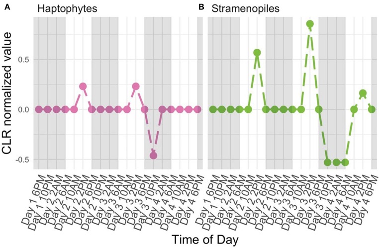
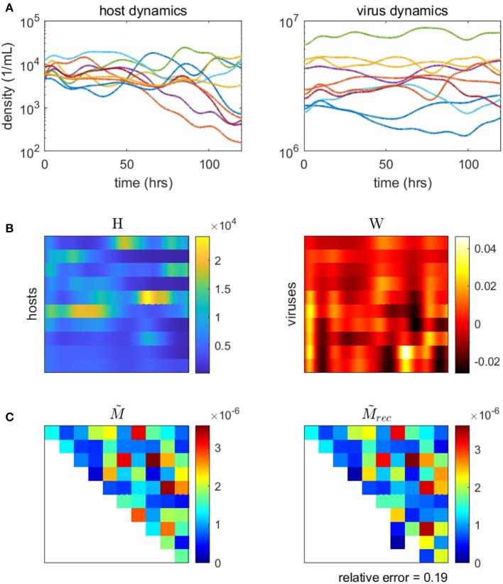
Time-series can provide critical insights into the structure and function of microbial communities. The analysis of temporal data warrants statistical considerations, distinct from comparative microbiome studies, to address ecological questions. This primer identifies unique challenges and approaches for analyzing microbiome time-series. In doing so, we focus on (1) identifying compositionally similar samples, (2) inferring putative interactions among populations, and (3) detecting periodic signals. We connect theory, code and data via a series of hands-on modules with a motivating biological question centered on marine microbial ecology. The topics of the modules include characterizing shifts in community structure and activity, identifying expression levels with a diel periodic signal, and identifying putative interactions within a complex community. Modules are presented as self-contained, open-access, interactive tutorials in R and Matlab. Throughout, we highlight statistical considerations for dealing with autocorrelated and compositional data, with an eye to improving the robustness of inferences from microbiome time-series. In doing so, we hope that this primer helps to broaden the use of time-series analytic methods within the microbial ecology research community.

Keywords: clustering; code:R; code:matlab; inference; marine microbiology; microbial ecology; periodicity; time-series analysis.

Figure 1

Independent random walks yield apparently significant correlations (when evaluated as independent pairs) despite no underlying interactions, in contrast to residuals (i.e., point-to-point differences). (A) Time-series of independent random walks, x_i(t). (B) Correlation structure of independent random walks. (C) Distribution of correlation values for an ensemble of independent random walks, with p-value = 0.05 marked (red lines). (D) Time-series of the residuals of independent random walks, i.e., Δx_i(t) = x_i(t + Δt) − x_i(t). (E) Correlation structure of residual time-series. (F) Distribution of correlation values for the same ensemble as (C) but taken between the residual time-series, with p-value = 0.05 marked (red lines).

Figure 2

Workflow of techniques implemented in each module. The top layer considers questions of interest for a particular study. In the second layer, data normalizations are listed as implemented in module I and module II. For module III, we use synthetic data and instead list modeling inputs. The third layer shows the analytical techniques used in this primer, which we note is not exhaustive. These techniques provide some insight into the initial question asked, as described in the fourth layer.

Figure 3

Comparing statistical ordination techniques for 18S community compositions across samples. (Top row) Ordinations using Jaccard distance for comparison of presence/absence of community members between samples. (Bottom row) Ordinations using Euclidean distance on isometric log-ratio transformed data. (A,D) Non-metric Multidimensional Scaling (NMDS) projection in two dimensions, arbitrary units. Convex hulls have been drawn to emphasize ordinal separation of 6 AM (yellow), 10 AM (light green), and 2 PM (teal) samples. (B,E) Scree plots for PCoA ordinations. Each bar corresponds to one axis of the PCoA, the height is proportional to the amount of variance explained by that axis. We decided the first 3 axes were necessary to summarize the data in these cases [explaining a total of (B) 64.76% and (E) 37.54% of the variance]. Shading of bars indicate our interpretations of which axes are important to show (black), which are unimportant (light gray), and which are intermediate cases (medium gray). (C,F) PCoA ordinations using the selected axes after scree plot examination. Each point is one sample, the color of the point indicates the time of day at which the sample was taken (colors correspond to NMDS projections).

Figure 4

Characterization of protist clusters. (A) Cluster membership based on the phylum or class level protistan taxonomy. The “Other/unknown” category includes sequences with non-specific identity, such as “uncultured eukaryote” and “Unassigned” denotes sequences with no taxonomic hit (< 90% similar to reference database). (B) Representative taxon time-series for each cluster. Y-axis is z-score (see Methods: Normalizations), so a value of 0 corresponds to mean expression level. White and shaded regions represent samples taken during the light (white) dark cycle (shaded).

Figure 5

Centered Log Ratio (CLR)-transformed, detrended 18S rRNA gene levels (y-axes) over time (x-axes) for a subset of OTUs found to have significant diel periodicity (RAIN analysis). A value of 0 denotes the mean expression level for a given OTU. Included OTUs belong to the (A) Haptophyte and (B) Stramenopile groups. White and shaded regions represent samples taken during the light (white) dark cycle (shaded).

Figure 6

Inferring the microbe-virus infection network from time-series data for a 10 by 10 synthetic microbe-virus community. (A) Simulated host (left) and virus (right) densities over time. (B) Host densities (left, H) and transformed virus differences (right, W), for input into the objective function (Equation 20). (C) The original “ground-truth” interaction network (left) and the reconstructed network (right). In the interaction matrix, the rows denote hosts, the columns represent viruses, and the colors denote the scaled intensity of interactions (where white denotes no interaction).

References

1. Agrawal A., Verschueren R., Diamond S., Boyd S. (2018). A rewriting system for convex optimization problems. J. Control Decis. 5, 42–60. 10.1080/23307706.2017.1397554 - DOI
1. Aitchison J. (1983). The statistical analysis of compositional data. J. Int. Assoc. Math. Geol. 44, 139–177.
1. Aitchison J. A., Vidal C., Martín-Fernández J., Pawlowsky-Glahn V. (2000). Logratio analysis and compositional distance. Math. Geol. 32, 271–275. 10.1023/A:1007529726302 - DOI
1. Aylward F. O., Boeuf D., Mende D. R., Wood-Charlson E. M., Vislova A., Eppley J. M., et al. . (2017). Diel cycling and long-term persistence of viruses in the ocean's euphotic zone. Proc. Natl. Acad. Sci. U.S.A. 114, 11446–11451. 10.1073/pnas.1714821114 - DOI - PMC - PubMed
1. Aylward F. O., Eppley J. M., Smith J. M., Chavez F. P., Scholin C. A., DeLong E. F. (2015). Microbial community transcriptional networks are conserved in three domains at ocean basin scales. Proc. Natl. Acad. Sci. U.S.A. 112, 5443–5448. 10.1073/pnas.1502883112 - DOI - PMC - PubMed
LinkOut - more resources