Hippocampal Network Reorganization Underlies the Formation of a Temporal Association Memory

Abstract

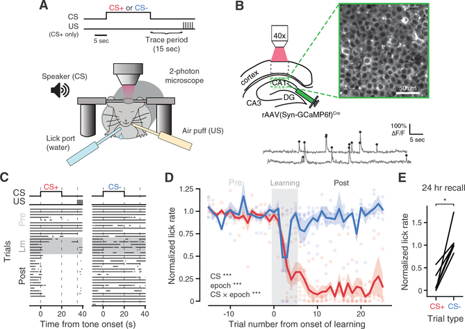
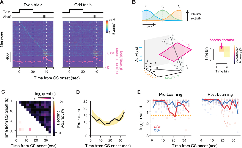
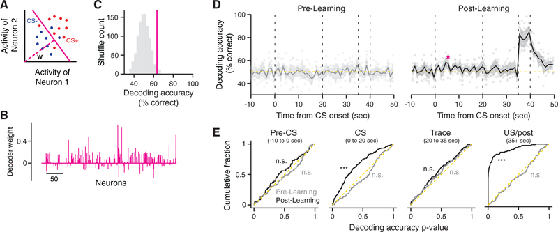
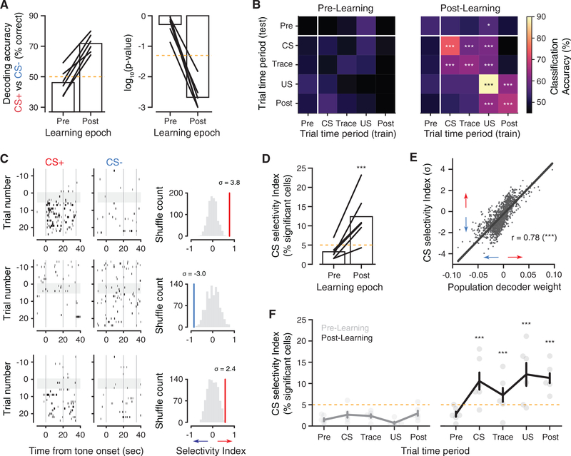
Episodic memory requires linking events in time, a function dependent on the hippocampus. In "trace" fear conditioning, animals learn to associate a neutral cue with an aversive stimulus despite their separation in time by a delay period on the order of tens of seconds. But how this temporal association forms remains unclear. Here we use two-photon calcium imaging of neural population dynamics throughout the course of learning and show that, in contrast to previous theories, hippocampal CA1 does not generate persistent activity to bridge the delay. Instead, learning is concomitant with broad changes in the active neural population. Although neural responses were stochastic in time, cue identity could be read out from population activity over longer timescales after learning. These results question the ubiquity of seconds-long neural sequences during temporal association learning and suggest that trace fear conditioning relies on mechanisms that differ from persistent activity accounts of working memory.

Keywords: calcium imaging; hippocampus; learning; memory; population coding; trace fear conditioning.

Figure 1.. Two-Photon Functional Imaging of CA1 Pyramidal Neurons during Differential tFC

(A) Schematic of experimental paradigm. A head-fixed mouse is immobilized and on each trial exposed to an auditory cue (CS+ or CS−) for 20 s, followed by a 15 s stimulus-free “trace” period, after which the US is triggered (CS+ trials). Air puffs are used as the US and lick suppression as a measure of learned fear. Operant water rewards are available throughout all trials. (B) Top, schematic of in vivo imaging with two-photon field of view in dorsal CA1. Bottom: calcium traces (gray) and inferred event times (black) from an example neuron. (C) Behavioral data for an example mouse over the complete paradigm. Each row is a trial, where dots indicate licks. (D) Summary of behavioral dataset. We compute a normalized lick rate for each trial by dividing the lick rate during the tone (0–20 s) by the rate in the pre-CS (−10 to 0 s) period (mean ± SEM; n = 6 mice; linear mixed-effects model with fixed effects of CS and learning epoch, with mouse as random effect; main effect significance shown in inset; post hoc models fit to each epoch separately with fixed effects of CS and trial number; Pre-Learning: no significant effects; Learning: effect of trial number [***] and CS × trial number [**]; Post-Learning: effect of CS [***]; Wald χ² test). Scatter shows data from individual mice. (E) Mean 24 h recall licking responses to first CS cue presentations of each day in the Post-Learning period for each mouse (n = 6 mice; Wilcoxon signed-rank test). *p < 0.05, **p < 0.01, and ***p < 0.001.

Figure 2.. Temporal Dynamics of CA1 Activity during tFC

(A) Summary of neural activity during Post-Learning CS+ trials, shown separately for even- and odd-numbered trials. Activity is trial averaged and sorted byneurons’ peak firing rate latency during 0–40 s in even trials. The population average event rate is overlaid. (B) Schematic of time decoding analysis. Top: trial-averaged tuning curves of a hypothetical sequence of time cells. Bottom: state space representation of theneural data. Dots indicate the neural state on single trials at three time points in the task. Right: a separate support vector machine (SVM) was trained to discriminate between population activity from every pair of time points in the task. (C) Matrix of classifiers for an example mouse during Post-Learning CS+ trials. Each square is the classifier result for comparing the pair of time bins corresponding to the x- and y-axis positions. The upper triangle reports the cross-validated accuracy, while the lower triangle reports the p value relative to a shuffle distribution. Most pairwise classifiers perform at chance level. (D) Time prediction performance for the example shown in (C). For each time bin in a test trial, all classifiers vote to determine the decoded time. Decodingaccuracy is the absolute error between real and predicted time. Black, cross-validated average of time decoding error. Yellow shading, 95% bounds of the null distribution. Decoding error is within chance levels throughout the trial. (E) Summary of decoding significance relative to the null distribution during Pre-Learning and Post-Learning trials. Bold lines are combined p values across micevia Fisher’s method. Red dashed line is the example shown in (C) and (D). Scatter shows individual p values across mice. Gold dashed line indicates p = 0.05.

Figure 3.. CS Identity Is Not Persistently Encoded in the Moment-to-Moment Activity of CA1

(A) Schematic of CS decoding analysis. A separate classifier was trained to discriminate between CS+ and CS− trials using population activity at each time point during the task (1 s bins). (B) Neuron weights for an example population decoder learned from Post-Learning data (averaged over cross-validation folds). (C) Accuracy of the decoder shown in (B). Purple line, average cross-validated decoding accuracy. Gray histogram, accuracy distribution obtained under surrogate datasets with shuffled trial labels. (D) CS decoding accuracy during Pre-Learning (left) and Post-Learning (right) trials. Data are presented as mean ± SEM across mice. Scatter shows average cross-validated decoding accuracy of individual mice at each time point. The example shown in (B) and (C) is marked in purple. (E) Cumulative distribution of decoding p values (calculated relative to shuffled data), shown separately for each trial time period. Dashed yellow line indicates the uniform distribution (chance, one-sample Kolmogorov-Smirnov test against the uniform distribution). *p < 0.05, **p < 0.01, and ***p < 0.001.

Figure 4.. CS Identity Is Predicted by CA1 Activity Rates on Longer Timescales

(A) CS decoding accuracy for classifiers trained on the average activity within each trial’s CS and trace period. Left: percentage accuracy; right: p value from nulldistributions calculated as in Figure 3. Each line is the average cross-validated result from one mouse. (B) Decoding CS identity from average activity in each trial time period. Decoders are trained and tested across each possible pair of time periods. Accuracy isaveraged across mice, and p values are combined via Fisher’s method, with Bonferroni correction. (C) Raster plots of three simultaneously recorded CS-selective neurons (from average activity across CS and trace period). Right: Post-Learning CS selectivity index for each neuron, compared with null distributions generated by recomputing the index on data with shuffled trial labels. (D) Percentage of active cells with significant CS selectivity, computed from average activity across CS and trace periods. (E) Regression of Post-Learning CS selectivity index for each neuron with its population decoder weight from (A) (Pearson’s correlation). (F) Fraction of selective neurons, computed separately in each trial time period. Data are presented as mean ± SEM across mice. Scatter show values of individualmice. p values indicate significant binomial test against the null hypothesis of ≤5%, pooled across mice. *p < 0.05, **p < 0.01, and ***p < 0.001.

References

1. Amit DJ, and Brunel N (1997). Model of global spontaneous activity and local structured activity during delay periods in the cerebral cortex. Cereb. Cortex 7, 237–252. - PubMed
1. Aronov D, Nevers R, and Tank DW (2017). Mapping of a non-spatial dimension by the hippocampal-entorhinal circuit. Nature 543, 719–722. - PMC - PubMed
1. Bakhurin KI, Goudar V, Shobe JL, Claar LD, Buonomano DV, and Masmanidis SC (2017). Differential encoding of time by prefrontal and striatal network dynamics. J. Neurosci. 37, 854–870. - PMC - PubMed
1. Barak O, and Tsodyks M (2014). Working models of working memory. Curr. Opin. Neurobiol. 25, 20–24. - PubMed
1. Benna MK, and Fusi S (2016). Computational principles of synaptic memory consolidation. Nat. Neurosci. 19, 1697–1706. - PubMed
Publication types
LinkOut - more resources