. 2020 Nov;39(11):3379-3390.
doi: 10.1109/TMI.2020.2993835. Epub 2020 Oct 28.

Deep-Learning Image Reconstruction for Real-Time Photoacoustic System

Deep-Learning Image Reconstruction for Real-Time Photoacoustic System

MinWoo Kim et al. IEEE Trans Med Imaging. 2020 Nov.

Abstract

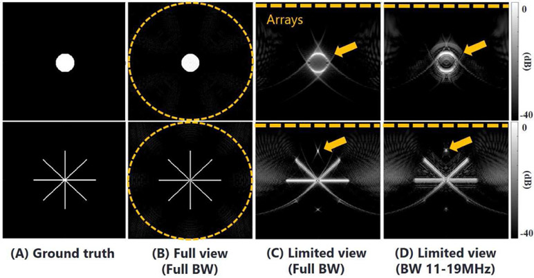
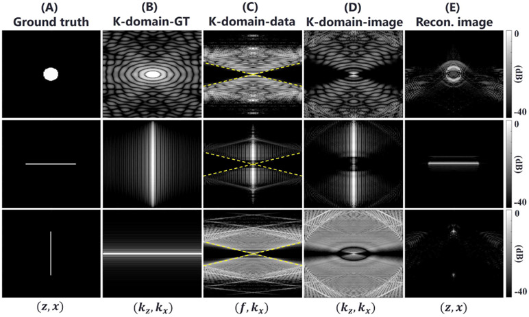
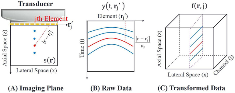
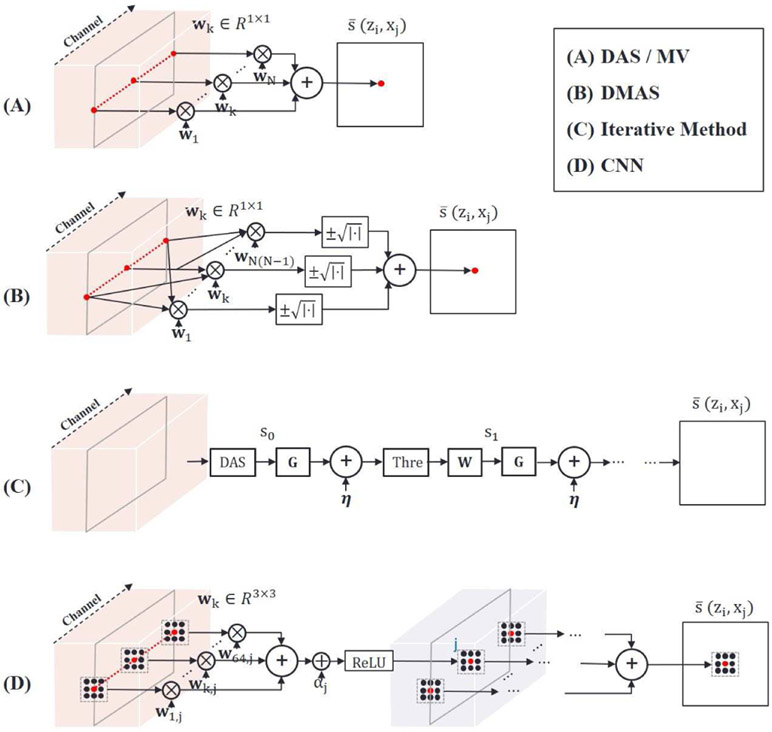
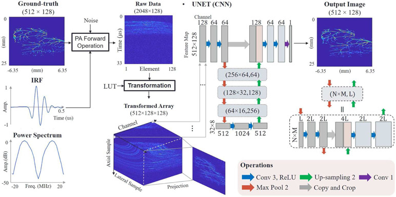
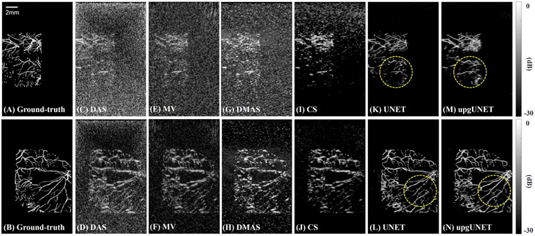
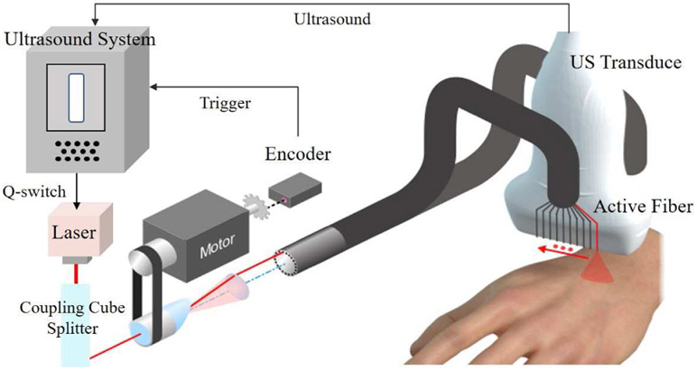
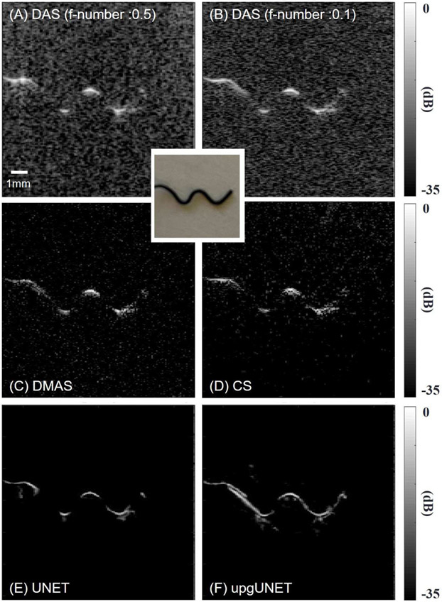
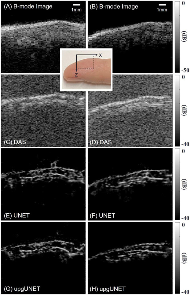
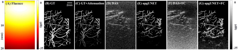
Recent advances in photoacoustic (PA) imaging have enabled detailed images of microvascular structure and quantitative measurement of blood oxygenation or perfusion. Standard reconstruction methods for PA imaging are based on solving an inverse problem using appropriate signal and system models. For handheld scanners, however, the ill-posed conditions of limited detection view and bandwidth yield low image contrast and severe structure loss in most instances. In this paper, we propose a practical reconstruction method based on a deep convolutional neural network (CNN) to overcome those problems. It is designed for real-time clinical applications and trained by large-scale synthetic data mimicking typical microvessel networks. Experimental results using synthetic and real datasets confirm that the deep-learning approach provides superior reconstructions compared to conventional methods.


Figures

Fig. 1.
Fig. 1.
Simulation results using standard filtered back-projection reconstruction. (A) presents two example object shapes. (B-D) shows reconstructions when the measurement conditions are (B) circular array with full bandwidth, (C) linear array with full bandwidth, and (D) linear array with limited bandwidth (11-19 MH). Arrows indicate structural losses and artifacts. All images are visualized on a log-scale colormap (40 dB range).
Fig. 2.
Fig. 2.
Reconstruction simulations in k-space using one circular object and two simple linear objects rotated by 90 degrees. All images visualize absolute pixel values on a log-scale colormap (40 dB range). The maximum value in each image is represented as pure white. (A) Ground-truth images. (B) K-domain-GT obtained by 2-D Fourier transforming the ground truth. (C) K-domain-data obtained by 2-D Fourier transforming raw data. Raw x-t data obtained with the forward model. The dotted lines indicate f = ckx. The empty region (f < ckx) corresponds to evanescent waves. (D) K-domain-image by nonlinear mapping of K-domain-data. (E) Reconstructed image obtained by 2-D inverse Fourier transforming K-domain-image.
Fig. 3.
Fig. 3.
(A) Measurement geometry. A 2-D image plane with respect to a linear array transducer is defined as the z-x plane. (B) 2-D measurement data. The curved lines indicate propagation delay profiles of particular image points at different depths. (C) 3-D transformed data. Channel packets correspond to the delay profiles indicated by straight lines.
Fig. 4.
Fig. 4.
Schematic diagram illustrating reconstruction methods. 2-D measurement data are transformed into a 3-D array as shown in Fig. 3 followed by reconstruction. (A) DAS / MV methods. An image pixel is determined by weighting and summing channel samples at a corresponding pixel position. Weights vary with position. Unlike DAS, MV adaptively assigns weights depending on data statistics. (B) DMAS method. Channel samples are coupled and multiplied before summation. This additional nonlinear operation is required to prevent a dimensional problem. (C) Iterative method. This is based on the L1 minimization problem in compressed sensing (CS). The initial solution is ordinarily obtained by DAS. The solution is updated by matrix multiplications, matrix additions, and threshold operations. (D) Basic structure of CNN. It applies convolution with a 3 × 3 kernel to multi-channel inputs, and returns multi-channel outputs. The full network consists of multiple layers, where each layer contains the convolution operation, bias addition and Rectified Linear Unit (ReLU) operation to enhance expressive power.
Fig. 5.
Fig. 5.
Deep-learning architecture for PA image reconstruction. Raw data are converted into a 3-D array by a lookup table (LUT). The array is used as a multi-channel input to the network (first box). Each box represents a multi-channel feature map. The number of channels is denoted on the top or bottom of the box. Feature map sizes decrease and increase via max-pooling and upsampling, respectively. All convolutional layers consist of 3 × 3 kernels except the last layer. The network is trained by minimizing the mean squared error between output images and ground-truth images.
Fig. 6.
Fig. 6.
Reconstruction results using synthetic data. Two particular objects are tested and all images are displayed using a log-scale colormap. (A,B) Ground-truth images. (C,D) Delay-and-sum results. Hilbert transform is applied as post-processing. (E,F) Minimum variance results. (G,H) Delay-multiply-and-sum results. (I,J) Iterative CS method results. Wavelet dictionaries and total-variation regularization are used for compressed sensing. (K,L) Deep-learning results. An input is a 2-D array using DAS. (M,N) Deep-learning results. An input is a 3-D multi-channel array.
Fig. 7.
Fig. 7.
Our customized PAUS system. An US scanner triggers a compact diode-pumped laser such that it emits pulses (around 1 mJ energy) at a 1 kHz rate with switching wavelength ranging from 700 nm to 900 nm. The laser is delivered to integrated fibers arranged on the two sides of a linear array transducer. A motor controlled by the scanner allows laser pulses to couple with different fibers sequentially. The scanner records PA signals that originate from light propagation into tissue.
Fig. 8.
Fig. 8.
Reconstruction results. All images are displayed using a log-scale colormap (35 dB range). A ‘W’ shape wire is scanned by the PAUS system. (A) Delay-and-sum result. The f-number is 0.5. (B) Delay-and-sum result. The f-number is 0.1. (C) Delay-multiply-and-sum results. (D) Iterative CS method results. (E) UNET deep-learning result. An input is a 2-D array using DAS. (F) upgUNET deep-learning result. An input is a 3-D multi-channel tensor.
Fig. 9.
Fig. 9.
In vivo reconstruction results. A human finger is scanned by the PAUS system. Two sagittal planes are tested. (A, B) US B-mode image. (C, D) Delay-and-sum result. The f-number is 0.5. (E, F) UNET deep-learning result. An input is a 2-D array using DAS. (G, H) upgUNET deep-learning result. An input is a 3-D multi-channel tensor. All images are displayed using a log-scale colormap. Mapping ranges for US and PD images are 50dB and 40dB, respectively.
Fig. 10.
Fig. 10.
Reconstruction results using synthetic data to explore penetration depth when PA signal attenuates with depth. One particular absorption object is tested and all images are displayed using a log-scale colormap. (A) Sum of light fluences from 20 fibers in a scattering medium. MCX Studio is used for the Monte Carlo simulation [44]. The details of the transducer geometry can be found Ref [1]. The effective attenuation coefficient of the medium is 1.73 cm−1. (B) Ground-truth object. (C) Attenuated object due to the heterogeneous fluence. Measurements are obtained from the object using Eq. 3. (D-G) Reconstruction results using (D) DAS, (E) deep-learning, (F) DAS with fluence compensation, and (G) deep-learning with fluence compensation.

Similar articles

Cited by

References

    1. Jeng G-S, Li M-L, Kim M, Yoon SJ, Pitre JJ, Li DS, Pelivanov I, and O’Donnell M, “Real-time spectroscopic photoacoustic/ultrasound (PAUS) scanning with simultaneous fluence compensation and motion correction for quantitative molecular imaging,” bioRxiv, 2019. - PMC - PubMed
    1. Attia ABE, Balasundaram G, Moothanchery M, Dinish U, Bi R, Ntziachristos V, and Olivo M, “A review of clinical photoacoustic imaging: Current and future trends,” Photoacoustics, p. 100144, 2019. - PMC - PubMed
    1. Schellenberg MW and Hunt HK, “Hand-held optoacoustic imaging: A review,” Photoacoustics, vol. 11, pp. 14–27, 2018. - PMC - PubMed
    1. Szabo TL, Diagnostic ultrasound imaging: inside out. Academic Press, 2004.
    1. Han SH, “Review of photoacoustic imaging for imaging-guided spinal surgery,” Neurospine, vol. 15, no. 4, p. 306, 2018. - PMC - PubMed

Publication types