Earth's water reservoirs in a changing climate

Abstract

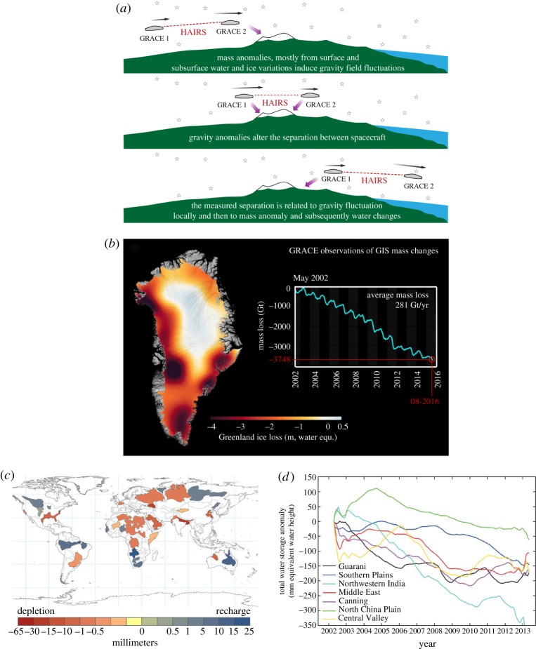
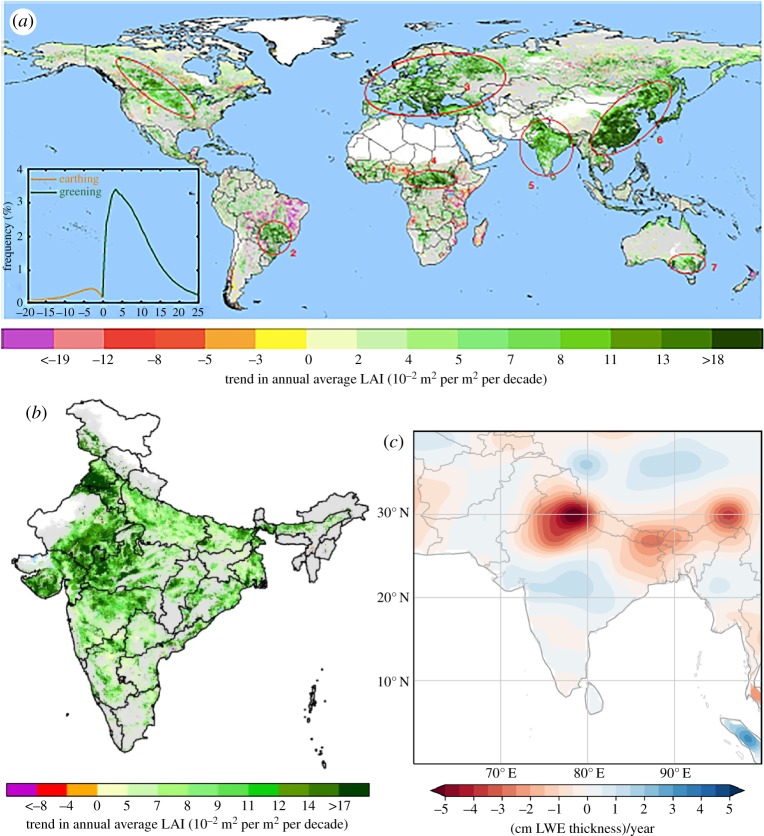
Progress towards achieving a quantitative understanding of the exchanges of water between Earth's main water reservoirs is reviewed with emphasis on advances accrued from the latest advances in Earth Observation from space. These exchanges of water between the reservoirs are a result of processes that are at the core of important physical Earth-system feedbacks, which fundamentally control the response of Earth's climate to the greenhouse gas forcing it is now experiencing, and are therefore vital to understanding the future evolution of Earth's climate. The changing nature of global mean sea level (GMSL) is the context for discussion of these exchanges. Different sources of satellite observations that are used to quantify ice mass loss and water storage over continents, how water can be tracked to its source using water isotope information and how the waters in different reservoirs influence the fluxes of water between reservoirs are described. The profound influence of Earth's hydrological cycle, including human influences on it, on the rate of GMSL rise is emphasized. The many intricate ways water cycle processes influence water exchanges between reservoirs and thus sea-level rise, including disproportionate influences by the tiniest water reservoirs, are emphasized.

Keywords: earth observations; reservoirs; water.

Figure 1.

Time series of global mean sea level (GMSL) recorded since 1992 from altimeter measurements on orbiting satellites [3]. This can be partitioned between changes in ocean mass derived from gravity fluctuation measurements from the space-borne gravity observing system (see box 1 and blue curve) and in ocean heat content derived from in situ measurements by ARGO floats (red). (Online version in colour.)

Figure 2.

(a) De-trended time series of sea-level rise to give sea-level anomalies (SLA_total), contribution to SLA of ocean water mass variations (SLA_mass) and sea surface salinity anomalies (SSSA) averaged between 50 N and 50S from the measurements of the SMOS satellite expressed in terms of practical salinity units (PSU). (b) Time series of SLA and latent heat flux anomalies (LH) averaged between 50 N and 50 S. The correlation between these two time series is −0.7 after 2012. (Online version in colour.)

Figure B1.

(a) The GRACE measurement approach: gravity field fluctuations, a result of surface and subsurface mass variations, are used to estimate the changes to water mass within Earth water reservoirs. (b) The systematic ice mass loss from Greenland over the GRACE observing period from 2002 to 2016. (c) GRACE groundwater storage annual trends for Earth's 37 largest aquifers for period 2003–2013 (from [10]). (c,d) Water storage declines (millimetre equivalent water height) in several of the world's major aquifers in Earth's arid and semi-arid mid-latitudes, derived from the NASA GRACE satellite mission. The monthly storage changes are shown as anomalies for the period April 2002–May 2013, with 24-month smoothing. (Online version in colour.)

Figure 3.

Earth's main water reservoirs and the fluxes of water between them. Also shown are known estimates of the change in these fluxes. All fluxes and estimates of change correspond to the period of the beginning of Earth observations and this period varies depending on the fluxes and studies that produce them. Updated from [,–18] and other sources including [19]. The flux changes, largely unknown, are denoted by Δ and those highlighted in red have an observational or physical basis underlying them. (Online version in colour.)

Figure B2.

Joint distributions of water vapour and its deuterium content (δD) in the lower troposphere (825–500 hPa) based on TES observations during the pre-transition stage (day −60 to −30, a), early transition (day 30–0, b), and the first 60 days of the Amazonian wet season (day 0–60, c). Simple models of evaporation and mixing from land and ocean (solid blue and black, respectively) as well as rainfall/Rayleigh models (dotted blue and black) are shown for comparison.

Figure 4.

The relation between zonal values of E-P and surface salinity (units are in practical salinity scale 1978 [34], after Wüst [33]. The solid line is the relation S (all seas) = 34.5 + 0.0175(E-P) also from [33].

Figure 5.

(a) A 58-year mean climatology of global sea surface salinity (SSS) after Durack & Wijffels [37]). (b–e) Four long-term estimates of global sea surface salinity (SSS) change, (b) from Durack & Wiffels ([37] analysis period 1950–2008), (c) Boyer et al. ([38]; analysis period 1955–1998), (d) Hosoda et al. ([39]; analysis period 1975–2005) and (e) Good et al. ([40]; analysis period 1950–2012) all scaled to represent equivalent magnitude changes over a 50-year period (practical salinity scale 1978, 50 yr^–1) (adapted from [41], fig. 2). (Online version in colour.)

Figure 6.

Evolution of GRACE (left column) and TRMM anomalies (right column) for six-month intervals during 2010 and 2011 when the GMSL dropped by almost 5 mm. Intervals shown for TRMM anomalies are offset by three months in order to provide context for changes in mass (fig. 3 of [47]).

Figure 7.

Time series of cumulative anomalies in SMB (blue), ice discharge (D, red) and total mass (M, purple = SMB-D) in Gt of (a) GIS and (b) AIS with uncertainties. Also shown are the equivalent sea-level rise contributions attached to this ice mass loss (recreated from both [56] and [49]). (Online version in colour.)

Figure 8.

Partitioned continental hydrologic fluxes according to [78], their figure 3. Terrestrial precipitation (annual mean± 1 s.d.) not intercepted by vegetation mixes into soils or flows into surface waters. Soil water is withdrawn by plant roots via transpiration, subjected to evaporation and leaks into the surface water. Of the flux entering the surface waters, 38% is derived from the soils, with the remainder being consistent with precipitation routed directly via preferential flow paths. Surface water that does not evaporate returns to the ocean as runoff. (Online version in colour.)

Figure 9.

Global mass budget estimate (fig. 3 of [48]) expressed as sea-level rise equivalent. The net of the land water storage is disaggregated into the contributions of SLR by land glaciers, human-driven changes (see text) and climate-driven water storage (including soil moisture changes and water storage). (Online version in colour.)

Figure B3.

(a) Global Map of trends in annual average MODIS leaf area index (AI) for 2000–2017. Statistically significant trends (Mann–Kendall test, p ≤ 0.1) are colour-coded. Grey areas show vegetated land with statistically insignificant trends. White areas depict barren lands, permanent ice-covered areas, permanent wetlands and built-up areas. Blue areas represent water. The highlighted greening areas in red circles mostly overlap with croplands, with the exception of circle number 4 [85]. (b) Expanded view of the trend in annual average LAI in croplands in India [85]. (c) GRACE record length trends (2002–2016) over the Indian subcontinent (in liquid water equivalent (LWE) units in cm per year), showing extensive groundwater depletion in Northwest India, as first described by Rodell et al. [86]. (Online version in colour.)

Figure 10.

(a) The regionally distributed slopes of the correlations between column water vapour change and sea surface temperature (SST) change (in % K⁻¹) over a 29-year period of sustained satellite water vapour and SST observations. (b) The distributions of the slopes the mean of the distributions. (Online version in colour.)

Figure 11.

(a) The annual frequency of ice and (b) water clouds over Greenland from joint CloudSat, CALIPSO observations. (c) The average relationship between mean liquid and ice water paths of clouds and the mean annual effect of these clouds on the surface radiation balance. This effect is positive at each location, indicative of the greenhouse effect, and increases with thicker clouds as the cloud water paths increase. (d) Evolution of GrIS SMB indicates that the cloudy simulations with an associated greenhouse effect have a lower SMB as a result of greater melt. Shaded areas indicate uncertainties (adapted from [104]). (Online version in colour.)

Figure B4.

(a) The A-Train constellation of satellites as in 2014. (b) An example of the profile of clouds and precipitation provided by the combination of lidar and radar through Typhoon Yuta on 10th of October 2018 clearly revealing the eye of the storm. The lidar provides a view of the upper thin clouds (orange) and the radar (yellows, reds and magenta) through deep clouds provide direct measure of cloud water, ice and rain. (c) The climatology of precipitation frequency of occurrence (expressed as a fraction) available from the CloudSat radar observations. Shown are the total occurrences from rain, drizzle and snow combined at 1 × 3 degree resolution derived from 10 years of space-borne radar observations.

Figure 12.

(a) Distribution of occurrence of daily 1°×1° accumulated precipitation over the tropical (30° S–30° N) land for the period 2012–2016. The colours correspond to various precipitation datasets listed on the right and described further in [122]. (b) The value of the 99.9th and 99th percentiles of the 1 × 1 daily accumulated tropical precipitation function of the 2 m daily temperature for a sub-set of the ensemble the observational products of (a). Shading is the standard deviation of the ensemble. The dashed-dot grey lines correspond to the C-C 6.5% K⁻¹ rate of change. (Online version in colour.)

References

1. O'Brien DP, Izidoro A, Jacobson SA, Raymond SN, Rubie DC. 2018. The delivery of water during terrestrial planet formation. Space Sci. Rev. 214, 47 (10.1007/s11214-018-0475-8) - DOI
1. Church JA, et al. 2013. Sea level change. In Climate change 2013: the physical science basis. Contribution of working group I to the fifth assessment report of the intergovernmental panel on climate change (eds Stocker TF, et al.). Cambridge, UK and New York, NY: Cambridge University Press.
1. Leuliette EW, Nerem RS. 2016. Contributions of Greenland and Antarctica to global and regional sea level change. Oceanography 29, 154–159. (10.5670/oceanog.2016.107) - DOI
1. Nerem RS, Chambers D, Choe C, Mitchum G. 2010. Estimating mean sea level change from TOPEX and Jason Altimeter Missions. Mar. Geod. 33(Suppl 1), 435–436. (10.1080/01490419.2010.491031) - DOI
1. Trenberth KE, Fasullo JT. 2010. Tracking earth's energy. Science 328, 316–317. (10.1126/science.1187272) - DOI - PubMed