Fluorescence lifetime imaging microscopy: fundamentals and advances in instrumentation, analysis, and applications

Abstract

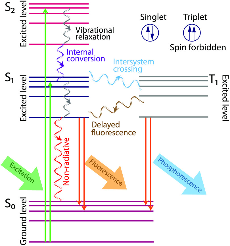
Significance: Fluorescence lifetime imaging microscopy (FLIM) is a powerful technique to distinguish the unique molecular environment of fluorophores. FLIM measures the time a fluorophore remains in an excited state before emitting a photon, and detects molecular variations of fluorophores that are not apparent with spectral techniques alone. FLIM is sensitive to multiple biomedical processes including disease progression and drug efficacy.

Aim: We provide an overview of FLIM principles, instrumentation, and analysis while highlighting the latest developments and biological applications.

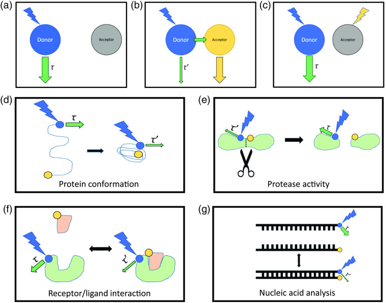
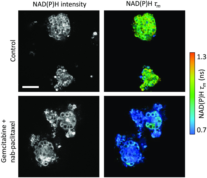
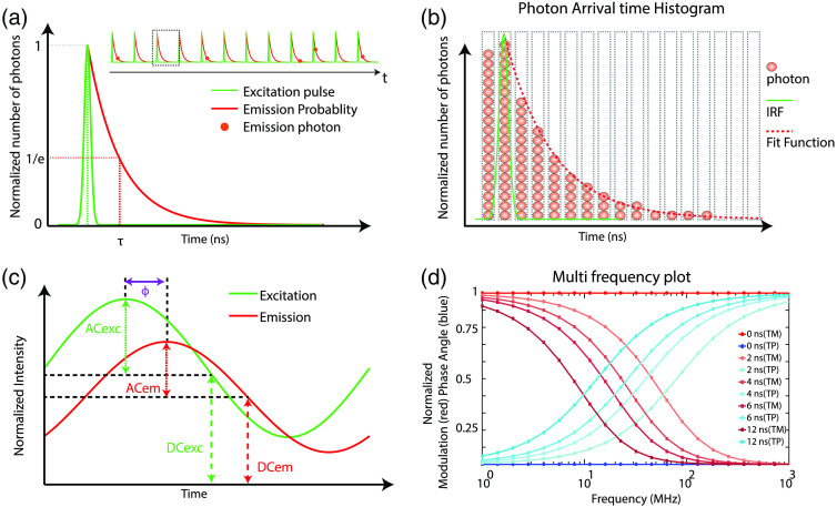
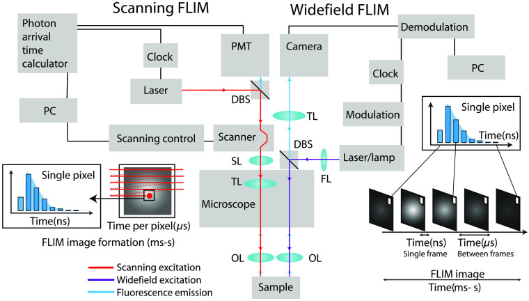
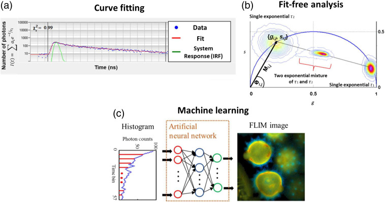
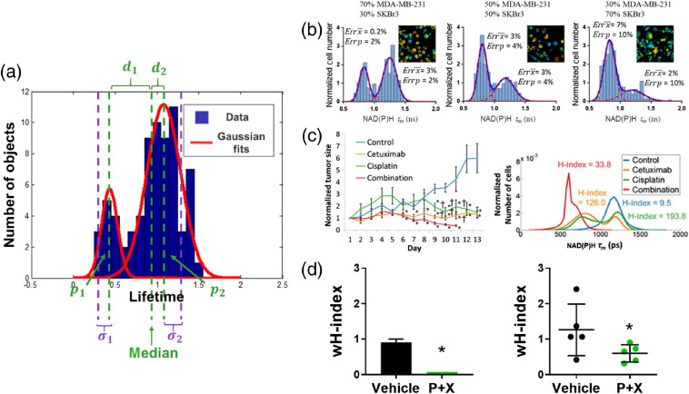
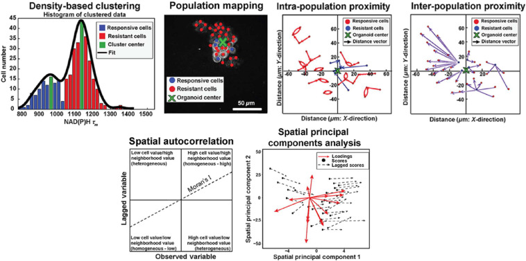
Approach: This review covers FLIM principles and theory, including advantages over intensity-based fluorescence measurements. Fundamentals of FLIM instrumentation in time- and frequency-domains are summarized, along with recent developments. Image segmentation and analysis strategies that quantify spatial and molecular features of cellular heterogeneity are reviewed. Finally, representative applications are provided including high-resolution FLIM of cell- and organelle-level molecular changes, use of exogenous and endogenous fluorophores, and imaging protein-protein interactions with Förster resonance energy transfer (FRET). Advantages and limitations of FLIM are also discussed.

Conclusions: FLIM is advantageous for probing molecular environments of fluorophores to inform on fluorophore behavior that cannot be elucidated with intensity measurements alone. Development of FLIM technologies, analysis, and applications will further advance biological research and clinical assessments.

Keywords: cell heterogeneity; fluorescence lifetime; image analysis; microscopy; review.

Fig. 1

Schematic of Jablonski diagram.

Fig. 2

FLIM-FRET concept and applications. (a) At the Förster distance (R₀, defined by the specific donor–acceptor pair), the efficiency of energy transfer between donor and acceptor is 50%, such that large distances exhibit low efficiencies of energy transfer. At these large distances, the fluorescence lifetime of the donor ($\tau$) is not affected by FRET. (b) As the distance between donor and acceptor decreases, FRET can occur, quenching the emission of the donor and shortening the donor lifetime decay (${\tau }^{\prime }$). (c) Photobleaching of the acceptor can confirm that the change in donor emission lifetime was due to a FRET interaction. (d), (e) Donor and acceptor pairs within the same molecule can be used to detect changes in (d) protein confirmation or (e) cleavage of proteins by proteases. (f), (g) Donor and acceptor pairs in separate molecules can be used to detect (f) receptor/ligand binding and (g) hybridization or splitting of nucleic acid strands.

Fig. 3

FLIM provides metabolic contrast in 3-D tumor organoids treated with chemotherapy. The ${\tau }_m$ of endogenous NAD(P)H is sensitive to the metabolic response to chemotherapy in patient-derived pancreatic cancer organoids. NAD(P)H intensity measurements alone did not distinguish treatment. Here, ${\tau }_m$ is calculated from a two-exponential decay of the free and protein-bound lifetimes of NAD(P)H. $\text{Scale bar}=50\mu \mathrm{m}$. Adapted with permission from Ref. .

Fig. 4

Schematic of time-domain (TCSPC) and frequency-domain FLIM. (a) TCSPC FLIM acquisition includes the short excitation pulse, single exponential fluorescence decay curve, and lifetime ($\tau$) defined at the $1/e$ value. Inset shows detected single fluorescence photons (red circles) at different time periods within multiple excitation pulses. (b) Photon time of arrival histogram built from the detection time of multiple fluorescent photons (red circles); green line represents the IRF, and dotted red line represents the fit function. (c) Schematic diagram of frequency-domain measurement with sinusoidally modulated excitation (exc) and the resulting phase shifted emission (em) signal. The AC and DC components of each signal are also indicated. (d) Modulation and phase versus frequencies for different lifetimes. TM, modulation lifetime; TP, phase lifetime.

Fig. 5

Schematic showing FLIM implementation in scanning and wide-field configurations. Two imaging modalities are compared side by side: scanning TCSPC FLIM and wide-field TG FLIM. The scanning beam of laser light from a galvanometric mirror is projected onto the back focal plane of the objective lens (OL) using the scan lens (SL) and tube lens (TL). The size of the beam and scan angle is often adjusted by varying the SL-TL pair. The light from the back focal plane is then focused by the objective lens into an excitation light cone. The emission from the same light cone is retraced back through a dichroic beamsplitter into a photon detector unit such as a photomultiplier tube (PMT). The electrical current from the PMT is amplified and read by an electronic board to calculate photon arrival times. These photon times are linked to the pixel of illumination by the computer (PC) that controls the scanner position in the image and thereby produces a histogram of photon arrival times for each pixel as shown in the inset of the left. LSM FLIM typically achieves 4 to 10 frames per second (fps) acquisition speed, which is usually limited by the scanner speed. (Right) Wide-field FLIM requires a focusing lens (FL) to achieve a field of illumination. The fluorescence from the focus of the objective lens is magnified by a tube lens and then imaged onto a camera sensor. FLIM in wide-field systems is achieved using a short frame exposure time (ns per frame). However, wide-field FLIM requires repeated frame acquisitions over a total time of milliseconds to seconds to collect sufficient photons for a complete histogram of fluorescence decay, as shown in the inset on the right side. Recent FLIM cameras intelligently select modulation-demodulation waveforms to achieve faster FLIM frame rates of $\sim 15\mathrm{fps}$.

Fig. 6

Examples of fluorescence lifetime estimation methods. (a) Curve fitting analysis determines lifetime decay variables $({\alpha }_i,{\tau }_i)$ by fitting an estimated decay function and estimated or measured IRF to experimental data. This process is iterated with the measured data to optimize goodness-of-fit parameters (${\chi }^2$). (b) Fit-free methods for estimating lifetime parameters of time-domain or frequency-domain lifetime data also exist. The phasor approach is one such technique frequently used for intuitive representation of fit-free lifetime estimation. Here, measured lifetime data can be transformed into phasor space to visualize pixels with similar lifetime values [Eqs. (12)–(15)]. Universal circle shown as blue semicircle. Example phasors for single exponential species $({\tau }_1,{\tau }_2)$ and a two-component mixture of ${\tau }_1$ and ${\tau }_2$ illustrate the rule of linear addition. (c) Neural networks can be trained with simulated or experimental FLIM data for fast generation of fluorescence lifetime maps. Adapted under CC BY-4.0 with permission from Ref. .

Fig. 7

Heterogeneity analysis of fluorescence lifetime data. (a) Histograms of lifetimes per object are fit to distribution models to describe subpopulations and variability in the data. The $H$-index and $wH$-index are derived from these fits [Eqs. (19) and (20), respectively]. Here, $p_i$ is the proportion of each subpopulation, $d_i$ is the distance between subpopulation median and global median, and ${\sigma }_i$ is the subpopulation standard deviation. (b) Distribution density models fit to cell-level NAD(P)H mean lifetimes can accurately identify distinct breast cancer cell lines (MDA-MB-231 and SKBr3) in mixed cocultures (proportion of mixtures indicated above plots). Errors (Err) in the model predictions for mean ($\overline{x}$) and proportion ($p$) of each population are given within each plot. Adapted with permission from Ref. . (c) $H$-index of in vivo FaDu tumor cell NAD(P)H mean lifetime (right) correlates with in vivo treatment response (left). Adapted with permission from Ref. . (d) Cell autofluorescence $wH$-index is similar for (left) in vitro organoids derived from primary PyVmT tumors and (right) in vivo PyVmT tumors with vehicle and combination treatment. Adapted with permission from Ref. .

Fig. 8

Spatial analysis of fluorescence lifetime distribution. Spatial statistical analyses can quantify spatial heterogeneity in fluorescence lifetimes. Here, spatial heterogeneity in cell-level autofluorescence lifetimes is used as an example. (a) Density-based clustering defines cell subpopulations that are mapped back onto lifetime images. Relative proximity measurements define spatial distributions within (intrapopulation proximity) and between (interpopulation proximity) cell subpopulations. (b) Multivariate spatial heterogeneity is quantified with spatial autocorrelation and spatial principal components analysis. Adapted under CC BY-4.0 with permission from Ref. .

Fig. 9

Autofluorescence FLIM applications. (a) NAD(P)H FLIM of a mammary mouse tumor (heatmap) overlaid on an SHG image of collagen (grayscale). $\text{Scale bar}=100\mu \mathrm{m}$. Adapted with permission from Ref.  (b) Mean NAD(P)H lifetimes in solution and in the rat cortex in vivo after metabolic inhibition. [2DG, 2-deoxy-d-glucose; IAA, iodoacetic acid; KCNm, potassium cyanide; FCCP, carbonyl cyanide-4-(trifluoromethoxy)phenylhydrazone; BMI, bicuculline methiodide; ETC, electron transport chain.] * indicates significantly different from baseline in vivo measurement; Error bars indicate standard error across all pixels over all measurements. Reproduced with permission from Ref.  (c) Optical redox ratio [NAD(P)H/FAD; first row], NAD(P)H ${\tau }_m$ (second row), and FAD ${\tau }_m$ (third row) images of organoids generated from primary human breast tumors obtained from resection surgeries. TNBC, triple negative breast cancer; ER, estrogen receptor. $\text{Scale bar}=100\mu \mathrm{m}$. Adapted with permission from Ref. .

Fig. 10

Molecular probes for FLIM and FLIM-FRET. (a) Near-infrared fluorescence lifetime image of Cyp-GRD distribution (heatmap) in an A549-tumor-bearing mouse at 24-h postinjection. Adapted with permission from Ref.  (b) Fluorescence lifetime (heatmap) of mouse abdomen acquired 90 min after intravenous injection of LS-288. The low fluorescence lifetime region in the center of the abdomen is the filled urinary bladder. Adapted with permission from Ref. . (c) FLIM maps of the weighted mean fluorescence lifetime of T2AMPKAR-NES, a sensor for AMPK activation, in HEK293 spheroids. The blue end of the colormap indicates increased AMPK activation. $\text{Scale bar}=100\mu \mathrm{m}$. Adapted with permission from Ref. .

References

1. Stokes G. G., “On the change of refrangibility of light,” Philos. Trans. R. Soc. Lond. 142, 463–562 (1852).10.1098/rstl.1852.0022 - DOI
1. Jameson D. M., Ed., Perspectives on Fluorescence: A Tribute to Gregorio Weber, Springer International Publishing, Switzerland: (2016).
1. Chalfie M., et al. , “Green fluorescent protein as a marker for gene expression,” Science 263(5148), 802–805 (1994).SCIEAS10.1126/science.8303295 - DOI - PubMed
1. Inouye S., Tsuji F. I., “Aequorea green fluorescent protein: expression of the gene and fluorescence characteristics of the recombinant protein,” FEBS Lett. 341(2), 277–280 (1994).FEBLAL10.1016/0014-5793(94)80472-9 - DOI - PubMed
1. Stringari C., et al. , “In vivo single-cell detection of metabolic oscillations in stem cells,” Cell Rep. 10(1), 1–7 (2015).10.1016/j.celrep.2014.12.007 - DOI - PMC - PubMed
Publication types