Bayesian regression explains how human participants handle parameter uncertainty

Abstract

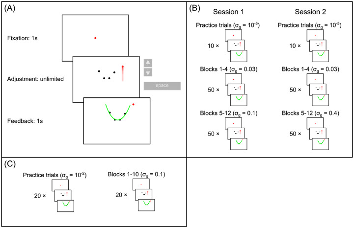
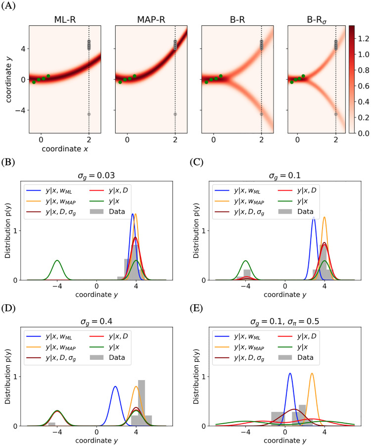
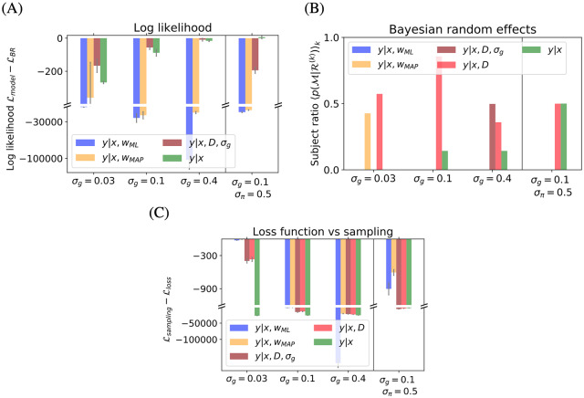
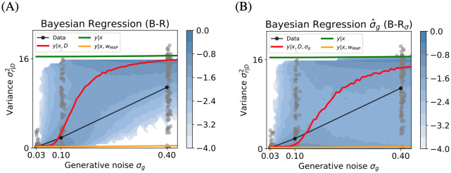
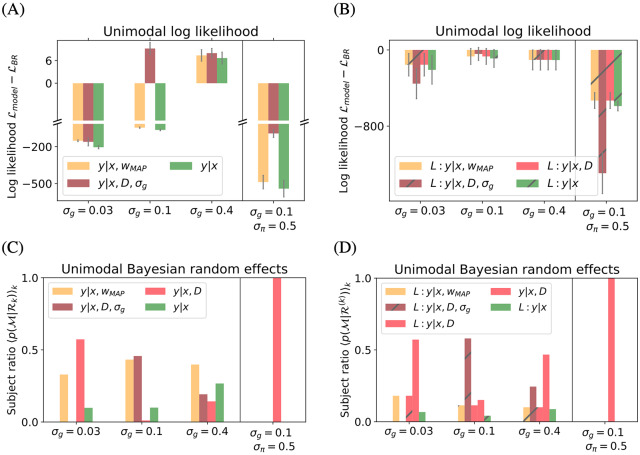
Accumulating evidence indicates that the human brain copes with sensory uncertainty in accordance with Bayes' rule. However, it is unknown how humans make predictions when the generative model of the task at hand is described by uncertain parameters. Here, we tested whether and how humans take parameter uncertainty into account in a regression task. Participants extrapolated a parabola from a limited number of noisy points, shown on a computer screen. The quadratic parameter was drawn from a bimodal prior distribution. We tested whether human observers take full advantage of the given information, including the likelihood of the quadratic parameter value given the observed points and the quadratic parameter's prior distribution. We compared human performance with Bayesian regression, which is the (Bayes) optimal solution to this problem, and three sub-optimal models, which are simpler to compute. Our results show that, under our specific experimental conditions, humans behave in a way that is consistent with Bayesian regression. Moreover, our results support the hypothesis that humans generate responses in a manner consistent with probability matching rather than Bayesian decision theory.

Fig 1. Experimental protocol.

(A): Procedure of a single trial. First, a fixation dot was presented for 1s before the 4-dot stimulus appeared. Observers then had unlimited time to adjust the fifth dot with the up and down arrow keys. They then clicked the space bar to confirm the final position of the adjustable dot. After the response, the generative parabola was shown for 1s as feedback. (B): Experiment 1: The experiment consisted of two sessions on two separate days. Both sessions began with 10 practice trials with virtually no noise (σ_g = 10⁻⁵), followed by 4 blocks of 50 trials of low noise (σ_g = 0.03). In session 1, the low noise blocks were followed by 8 blocks of 50 trials of medium noise (σ_g = 0.1), while in session 2, the low noise blocks were followed by 8 blocks of 50 trials of high noise (σ_g = 0.4). In total, each participant completed 400 trials per noise level, with 20 repetitions of 20 unique stimuli. In this experiment, σ_π was set to 0.1. (C): Experiment 2: the experiment consisted of a single session which began with 20 practice trials with very low noise (σ_g = 10⁻²), followed by 10 blocks of medium noise (σ_g = 0.1) trials. Each block consisted of 20 trials, with the generative parabola shown as feedback, as in Experiment 1. Half of the 200 trials consisted of stimuli which were presented just once, while the remaining 100 trials consisted of 10 repetitions of 10 unique stimuli. In this experiment, σ_π was set to 0.5. See Materials and methods for more details.

Fig 2. Example responses.

B-R is the only model that can explain the transition from unimodal response (at low noise, (B)) to bimodal response distribution (at high noise, (D)). (A) A sample stimulus (green dots) at high noise level (σ_g = 0.4). For this specific stimulus, contours indicate the response distributions predicted by ML-R, MAP-R, B-R and B-R_σ (not shown to the participant) at various x^⋆. At x^⋆ = 2, we recorded the participant’s responses (gray dots). The cross section at x^⋆ = 2 is shown in (D). (B—E) The predicted response distributions at x^⋆ = 2 of ML-R (blue), MAP-R (orange), B-R (red), B-R_σ (dark red), P-R (green) and observed responses (gray). As σ_g increases (B—D), the data becomes less informative. Consequently, and in accordance with B-R, the response distribution becomes more bimodal. (E) Due to the weak prior the predictions of B-R and B-R_σ respond more strongly to the data and diverge from the modes of P-R more stronlgy than in the previous conditions. The skewness of B-R_σ results from the mixture of both Gaussian components.

Fig 3. Model comparison.

The model comparison shows that the B-R model best explains the data (A, B) and that sampling-based decision models outperform loss-based decision models (C). (A) Difference in log likelihood with respect to B-R averaged over participants for different experimental conditions. Negative values mean that B-R wins the comparison. B-R is either winning (σ_g ∈ (0.03, 0.1)) or equivalent to P-R because the two coincide at high levels of parameter uncertainty (σ_g = 0.4 and σ_π = 0.5). (B) The expected likelihood of each model for a randomly selected participant shows what fraction of participants are best described by a model. Overall, B-R and B-R_σ describe the population best. (C) Log likelihood difference between a sampling and a loss-based decision model. Negative values favour sampling. At all other conditions and for all regression models, sampling explains the data better than loss-based decision models with exact inference. For B-R, B-R_σ and P-R, loss-based models do not predict bimodal responses. At low noise σ_g = 0.03, loss-based models underestimate the response variance. Error bars represent the SEM across participants.

Fig 4. Response variances of predicted and empirical distributions, as a function of generative noise.

B-R best explains the increase in response variance as a function of the generative noise σ_g. Variances of the empirical response distributions from all participants (gray dots, median: gray line) and predicted response distributions, corresponding to the two B-R variants (median: red line, log probability: heatmap). B-R (A) Interpolating between MAP-R and P-R, only the B-R variants capture the upward trend in the data. At σ_g = 0.4, B-R fails to account for the empirical responses with close-to-zero variances. (B) At σ_g = 0.4, B-R_σ predicts a bimodal variance distribution because, in trials with low noise estimates, the predicted response distribution is unimodal and thus variance is low. Because of these low-variance trials, the median of B-R_σ increases slower than the median of B-R and captures the empirical median better. Because ML-R and MAP-R behaved identically, the MAP-R represents both regression models.

Fig 5. Median of each of the bimodal response distribution variance components across all participants and stimuli.

(A) Predicted coefficient of positive mode as a function of the empirical coefficient (across all noise levels). ML-R behaves identically to MAP-R. Thus, the MAP-R curve represents both models. The shaded area shows the 40% and 60% quantiles. (B) Prefactor of bimodal contribution as a function of generative noise. Data jittered for visibility. (C) Unimodal contribution to the variance. Empirical variance computed on mode with majority of responses. (D) Mean dispersion. Only trials with bimodal responses included. As the stimulus becomes more noisy, human responses and B-R variants conform to the prior.

Fig 6. Unimodal model comparison.

The unimodal analysis confirms previous results: overall B-R with sampling wins the model comparison. (A) Differences in log likelihood on unimodal data, averaged over participants. Negative values mean that B-R wins. ML-R is omitted because its poor performance complicates visualisation. (A) B-R wins at σ_g = 0.03 and σ_π = 0.5, but not in the other conditions. (B) All models use the quadratic loss function to select responses, with response variance given by the motor noise ${\sigma }_m^2$. B-R with sampling explains the unimodal data best for most participants. High subject-level variability results in large errors (see S1 Text for a subject-level analysis). (C, D) The fraction of participants best described by a given model. At σ_g = 0.4, several models perform well. Error bars indicate SEM across participants.

References

1. Knill DC, Pouget A. The Bayesian brain: the role of uncertainty in neural coding and computation. TRENDS in Neurosciences. 2004;27(12):712–719. 10.1016/j.tins.2004.10.007 - DOI - PubMed
1. Vilares I, Kording K. Bayesian models: the structure of the world, uncertainty, behavior, and the brain. Annals of the New York Academy of Sciences. 2011;1224(1):22–39. 10.1111/j.1749-6632.2011.05965.x - DOI - PMC - PubMed
1. Friston K. The history of the future of the Bayesian brain. NeuroImage. 2012;62(2):1230–1233. 10.1016/j.neuroimage.2011.10.004 - DOI - PMC - PubMed
1. Rahnev D, Denison RN. Suboptimality in perceptual decision making. Behavioral and Brain Sciences. 2018;41:e223 10.1017/S0140525X18000936 - DOI - PMC - PubMed
1. Petzschner FH, Glasauer S. Iterative Bayesian estimation as an explanation for range and regression effects: a study on human path integration. Journal of Neuroscience. 2011;31(47):17220–17229. 10.1523/JNEUROSCI.2028-11.2011 - DOI - PMC - PubMed
Publication types