Artificial neural networks for magnetic resonance elastography stiffness estimation in inhomogeneous materials

Abstract

Purpose: To test the hypothesis that removing the assumption of material homogeneity will improve the spatial accuracy of stiffness estimates made by Magnetic Resonance Elastography (MRE).

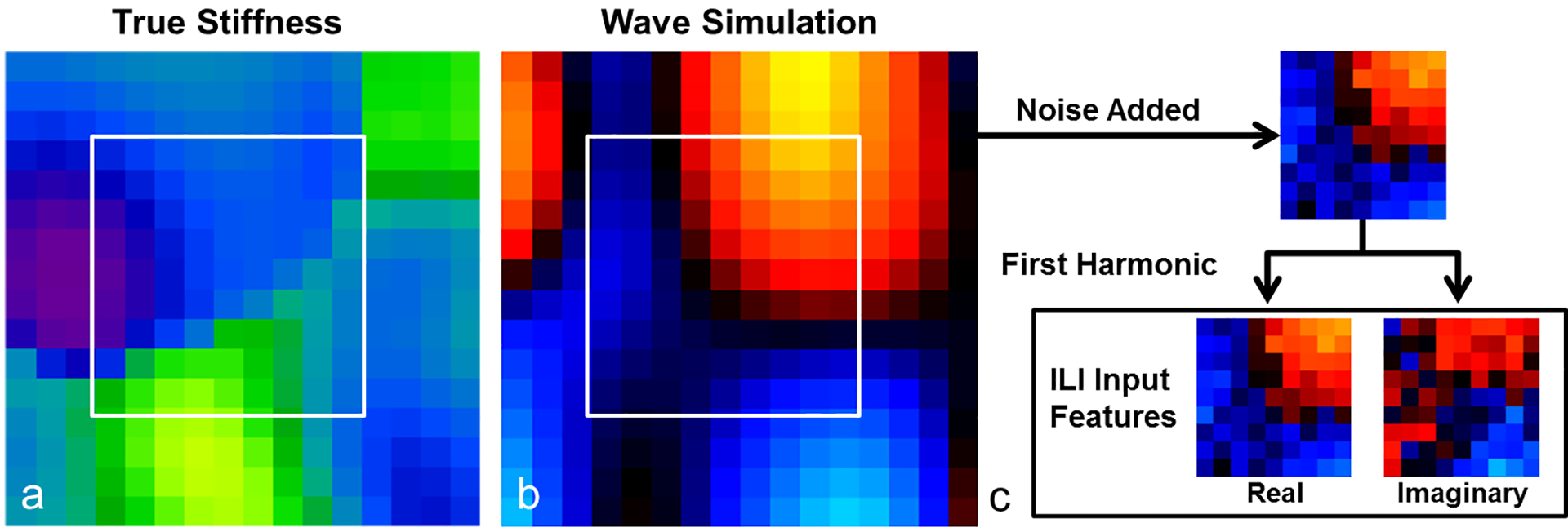
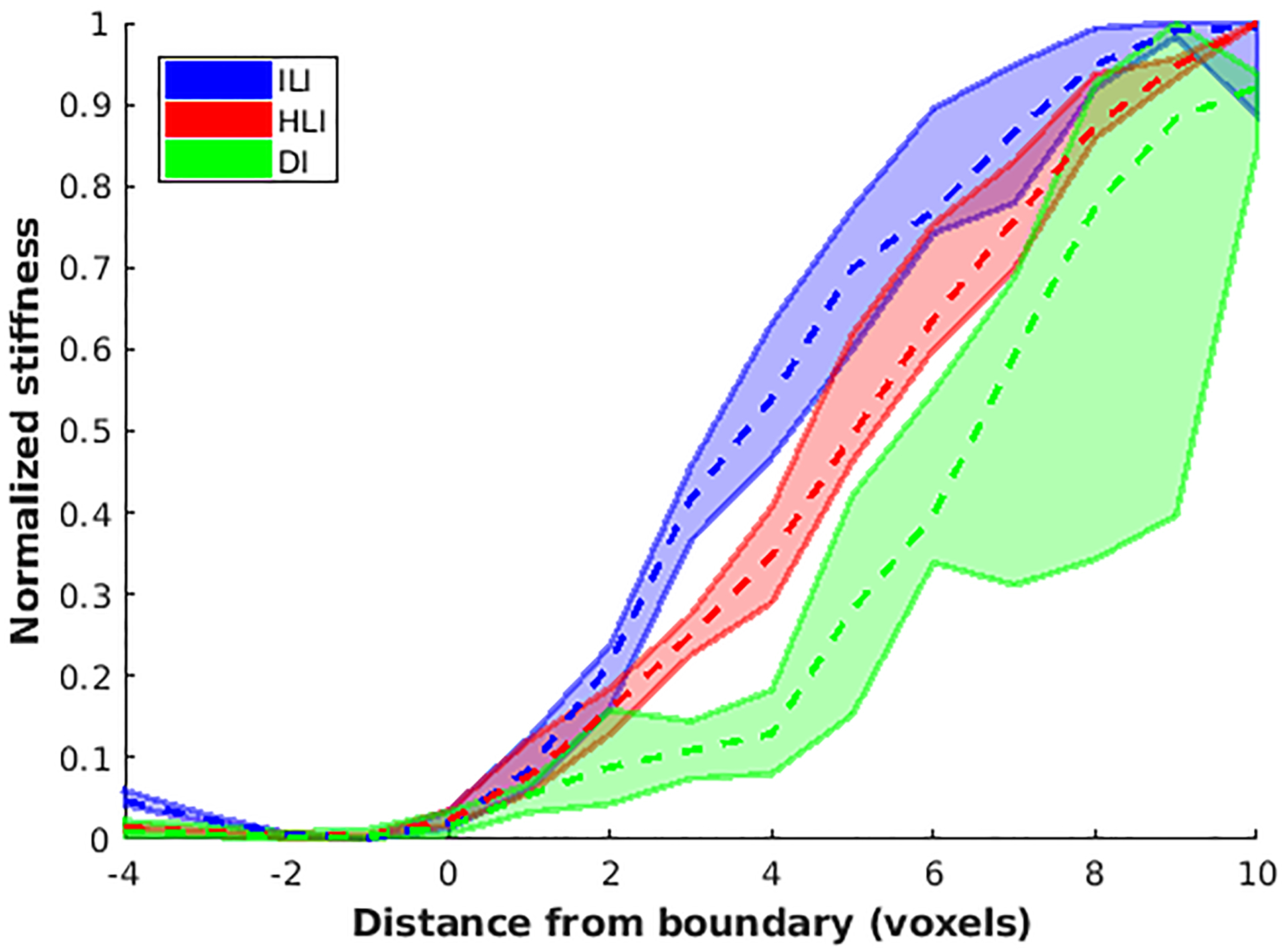
Methods: An artificial neural network was trained using synthetic wave data computed using a coupled harmonic oscillator model. Material properties were allowed to vary in a piecewise smooth pattern. This neural network inversion (Inhomogeneous Learned Inversion (ILI)) was compared against a previous homogeneous neural network inversion (Homogeneous Learned Inversion (HLI)) and conventional direct inversion (DI) in simulation, phantom, and in-vivo experiments.

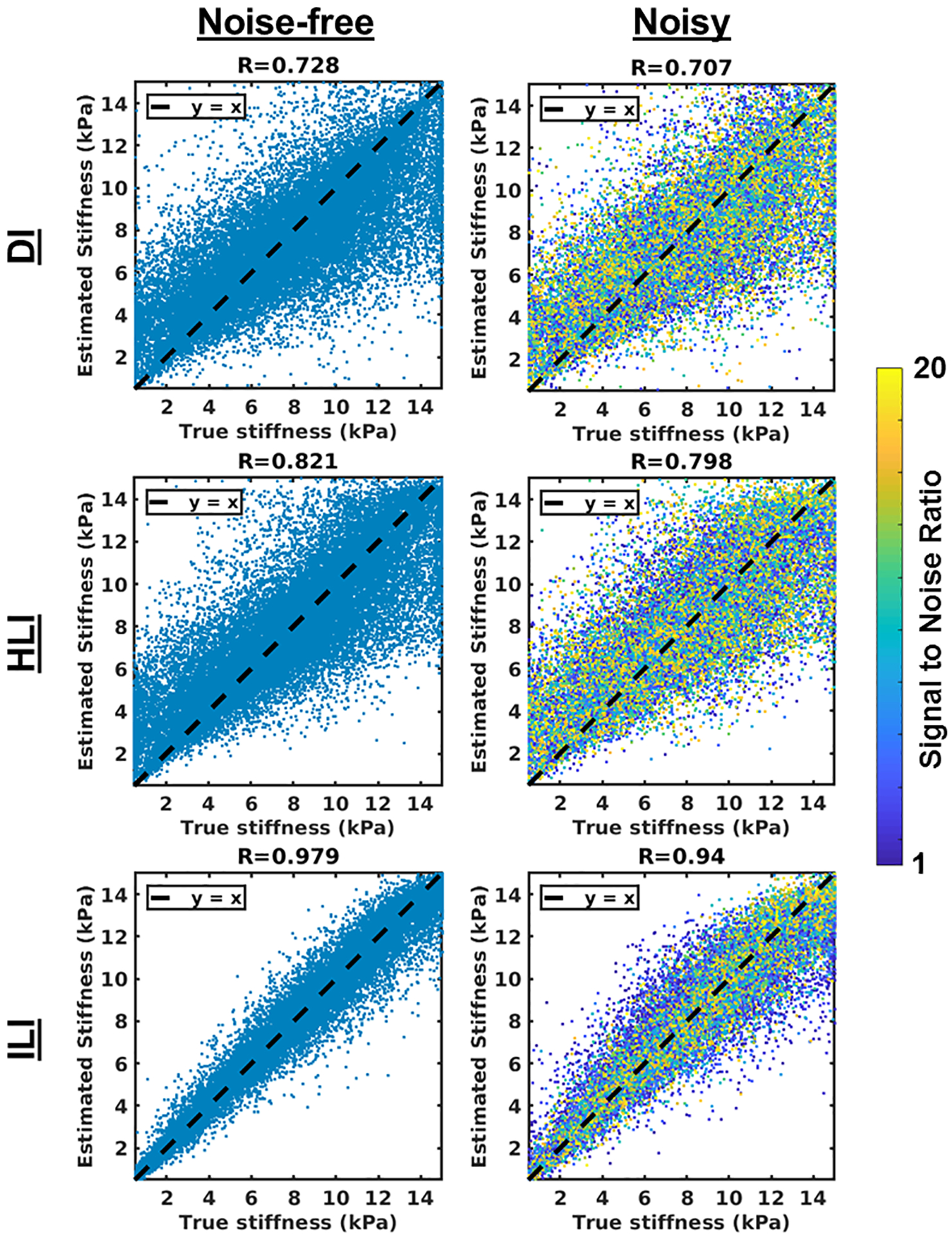
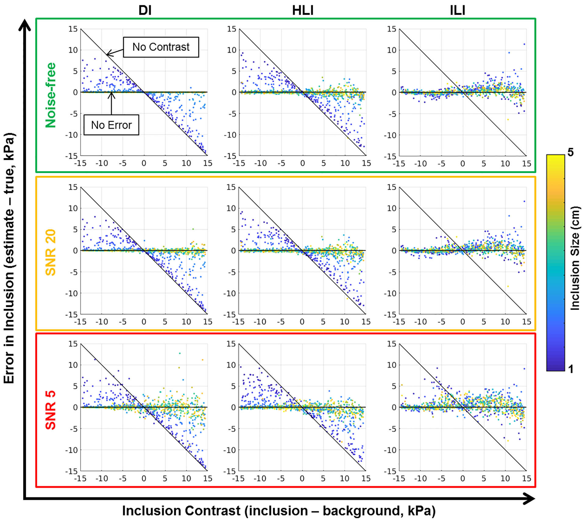
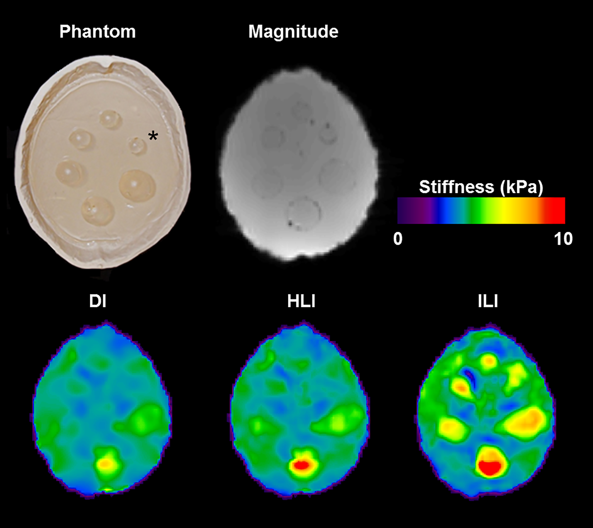
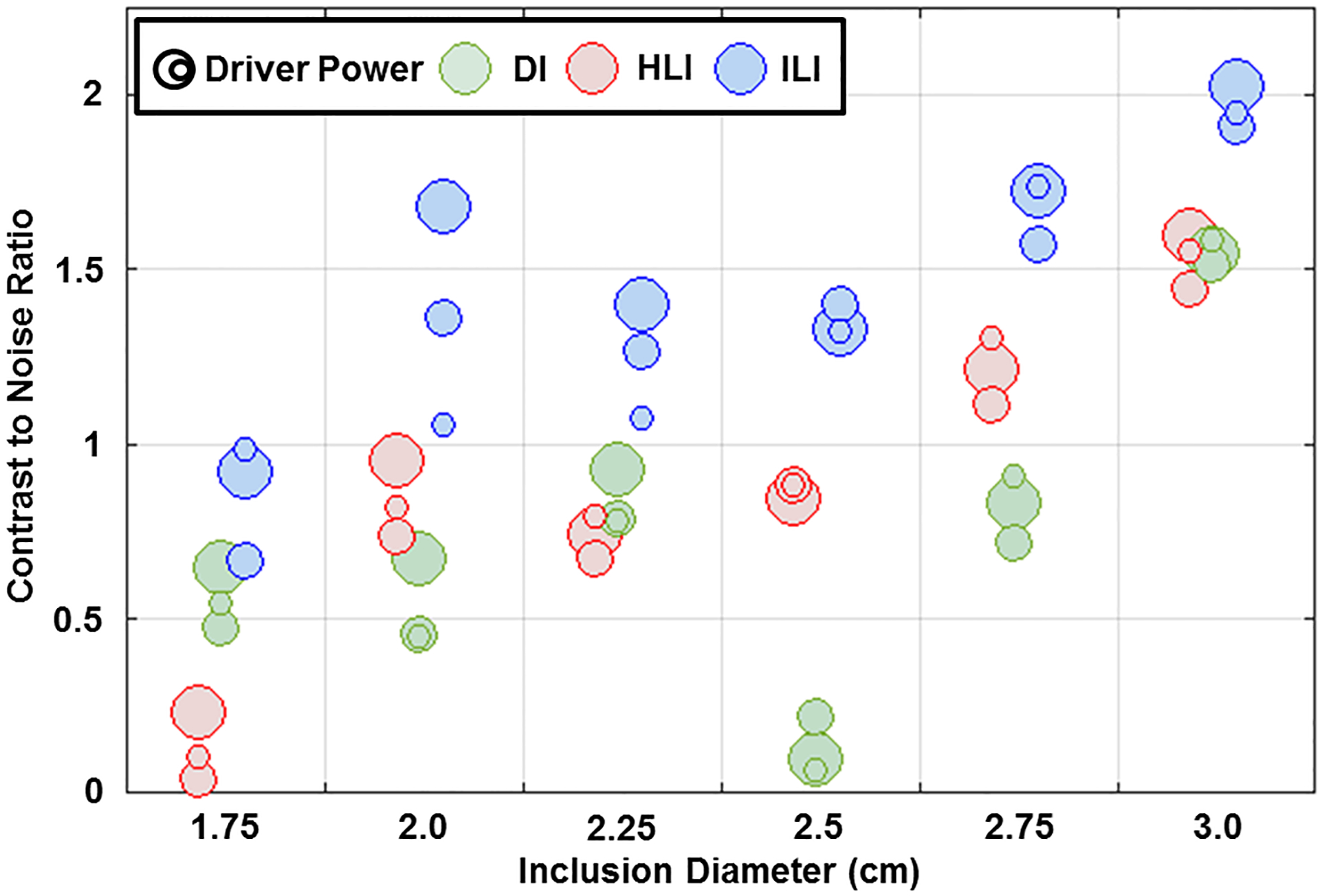
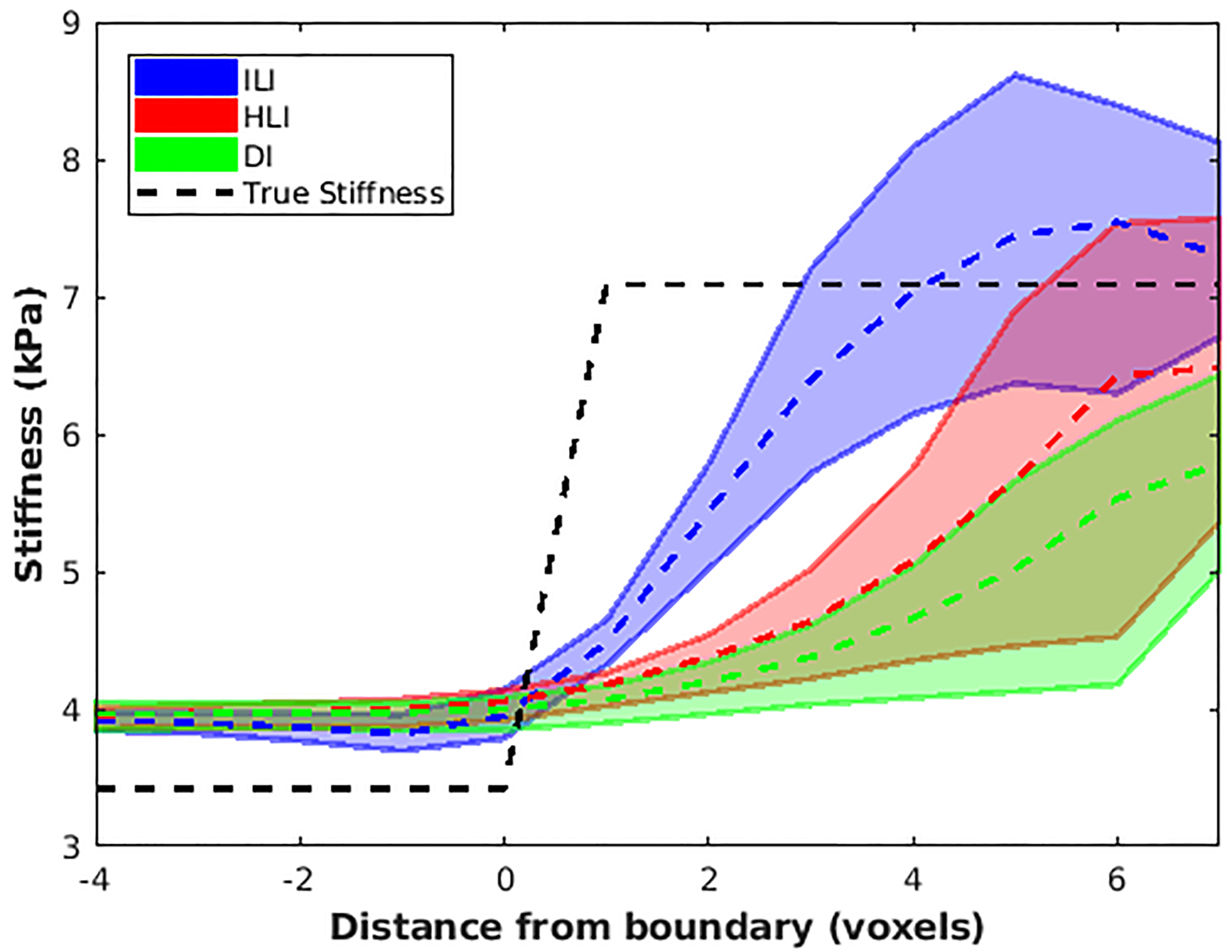
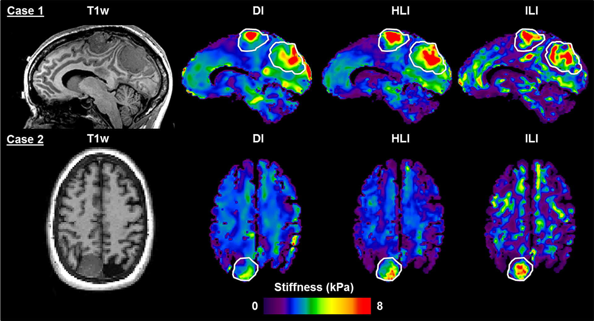
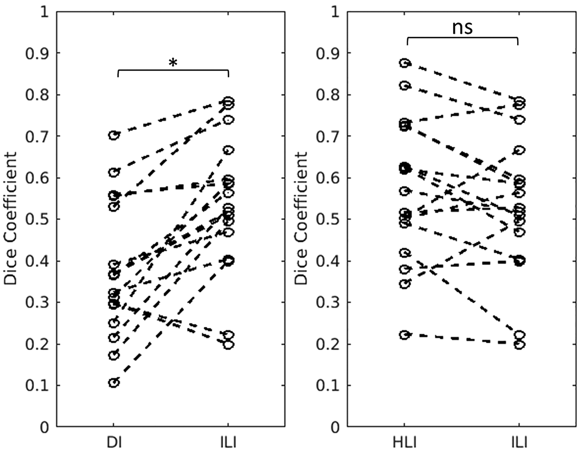
Results: In simulation experiments, ILI was more accurate than HLI and DI in predicting the stiffness of an inclusion in noise-free, low-noise, and high-noise data. In the phantom experiment, ILI delineated inclusions ≤ 2.25 cm in diameter more clearly than HLI and DI, and provided a higher contrast-to-noise ratio for all inclusions. In a series of stiff brain tumors, ILI shows sharper stiffness transitions at the edges of tumors than the other inversions evaluated.

Conclusion: ILI is an artificial neural network based framework for MRE inversion that does not assume homogeneity in material stiffness. Preliminary results suggest that it provides more accurate stiffness estimates and better contrast in small inclusions and at large stiffness gradients than existing algorithms that assume local homogeneity. These results support the need for continued exploration of learning-based approaches to MRE inversion, particularly for applications where high resolution is required.

Keywords: Artificial neural networks; Inversion; Magnetic resonance elastography; Stiffness.

Figure 1.. Summary of training data generation.

(a) Piecewise smooth input stiffness maps are generated by smoothing 3D Gaussian noise fields with 3D Gaussian kernels of randomly chosen x, y, and z dimensions. (b) Point-source wave sources are placed at the boundary of the simulation and the forward problem is solved to generate a wave image. (c) A 9×9×9 voxel patch, one such patch shown in the white square in (a) and (b), is taken from near the center of the simulation. The temporal first harmonic is taken after each patch has had noise added to generate the input features for the neural network.

Figure 2.. ILI is more accurate than HLI and DI in its test set.

DI, top row, HLI, middle row, and ILI, bottom row, results in a test set of 30,000 patches. Results for noise-free patches (first column) and noise added patches (second column) are shown. The spatial footprint that maximized the correlation coefficient in the noisy case is shown for each inversion (11×11×11 for DI, 9×9×9 for HLI, and 9×9×9 for ILI).

Figure 3.. Summary results from Coupled Harmonic Oscillators (CHO) experiment.

Each plot shows the error in inclusion estimate (estimated stiffness in the inclusion - true stiffness in inclusion) vs the inclusion contrast (true inclusion stiffness - true background stiffness) in 1000 CHO simulations. For a perfect inversion all points would be along the zero-error line. If an inversion completely fails to detect the inclusion points will be along the diagonal labeled “No Contrast”. The color of the data points corresponds to inclusion size.

Figure 4.. ILI more clearly depicts stiff inclusions in a brain-simulating phantom.

Top left: Photograph of the PVC phantom. Inclusion diameters, proceeding counter clockwise from the inclusion labeled with the asterisk, are 1.75, 2, 2.25, 2.5, 2.75, and 3cm. Top Middle: MRE magnitude image. Bottom left: Direct inversion after 3×3×3 median filtering. Bottom middle: HLI. Bottom right: ILI. The measured stiffness of the background and inclusions was 3.42 and 7.09 kPa, respectively.

Figure 5.. ILI provides higher contrast to noise ratio (CNR) in the phantom.

Calculated CNRs for the inversions shown in Figure 4. The size of the circles represents the driver power (3, 5 or 7 percent).

Figure 6.. ILI provides sharper transitions at inclusion boundaries.

Negative values on the x-axis represent distance from the boundary into the background while positive values show distance into the inclusion. Dashed lines connect median values at each position while solid lines show the 2.5^th and 97.5^th percentiles for each inversion.

Figure 7.. T1-weighted image and inversion results in two meningioma cases.

For Case 1, the superior tumor was described as stiff throughout and the posterior tumor was described as having heterogeneous stiffness on resection (only the superior tumor was included in group analysis). In Case 2, the tumor was described as very stiff throughout at resection. Regions of interest outline the tumor extent as manually traced on the T1-weighted image.

Figure 8.. Dice coefficient results in 17 meningioma cases.

ILI produces a significantly higher Dice coefficient than DI with 9×9×9 quartic smoothing. There is no significant difference between HLI and ILI Dice coefficients (p=0.15). Dashed lines connect the individual cases across the inversions. *p<0.001, ns = nonsignificant, two-tailed paired t-tests.

Figure 9.. ILI provides sharper transitions at boundaries of stiff tumors in vivo.

Negative values on the x-axis represent distance from the boundary into normal brain while positive values show distance into the tumor. The zero position is the first voxel labeled as tumor. Dashed lines connect median values at each position while solid lines show the 2.5th and 97.5th percentiles for each inversion.

References

1. Asbach P, Klatt D, Hamhaber U, Braun J, Somasundaram R, Hamm B, Sack I, 2008. Assessment of liver viscoelasticity using multifrequency MR elastography. Magn Reson Med 60, 373–379. 10.1002/mrm.21636 - DOI - PubMed
1. Ashburner J, Friston KJ, 2005. Unified segmentation. Neuroimage 26, 839–851. 10.1016/j.neuroimage.2005.02.018 - DOI - PubMed
1. Barnhill E, Davies PJ, Ariyurek C, Fehlner A, Braun J, Sack I, 2018. Heterogeneous Multifrequency Direct Inversion (HMDI) for magnetic resonance elastography with application to a clinical brain exam. Medical Image Analysis 46, 180–188. 10.1016/j.media.2018.03.003 - DOI - PubMed
1. Braun J, Buntkowsky G, Bernarding J, Tolxdorff T, Sack I, 2001. Simulation and analysis of magnetic resonance elastography wave images using coupled harmonic oscillators and Gaussian local frequency estimation. Magnetic Resonance Imaging 19, 703–713. 10.1016/S0730-725X(01)00387-3 - DOI - PubMed
1. Chollet Francois, 2015. Keras. https://keras.io.
Publication types