Geomorpho90m, empirical evaluation and accuracy assessment of global high-resolution geomorphometric layers

Abstract

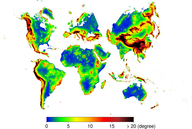
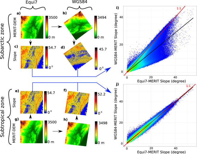
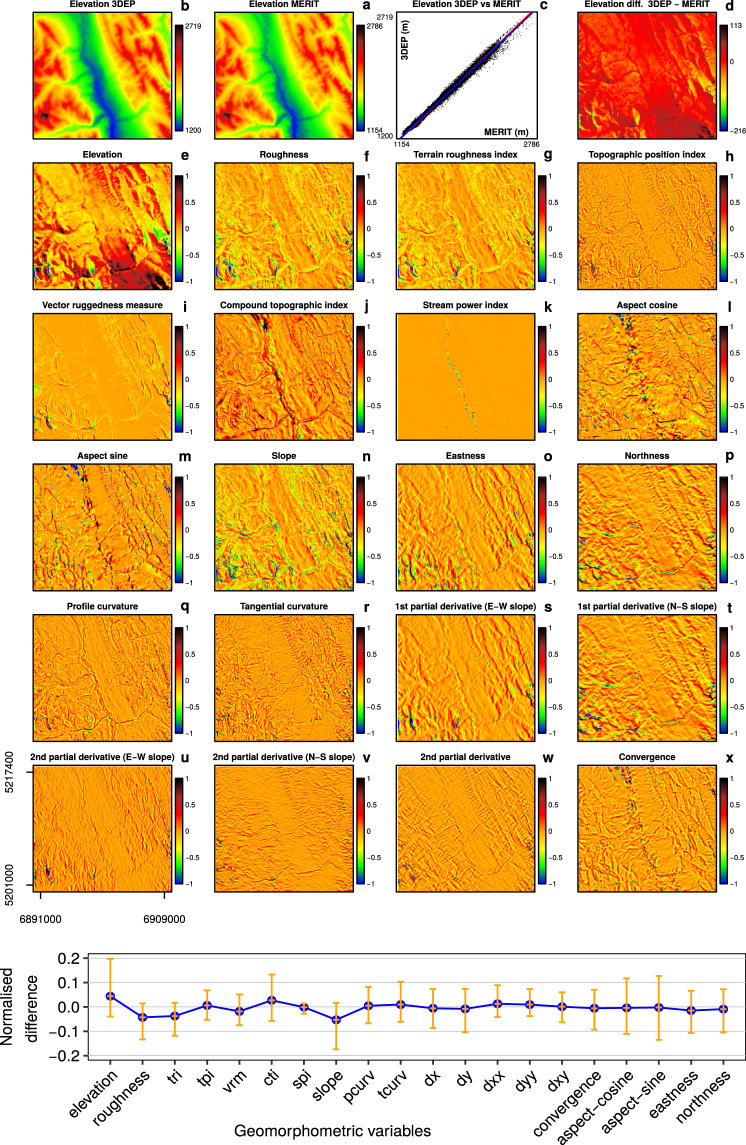
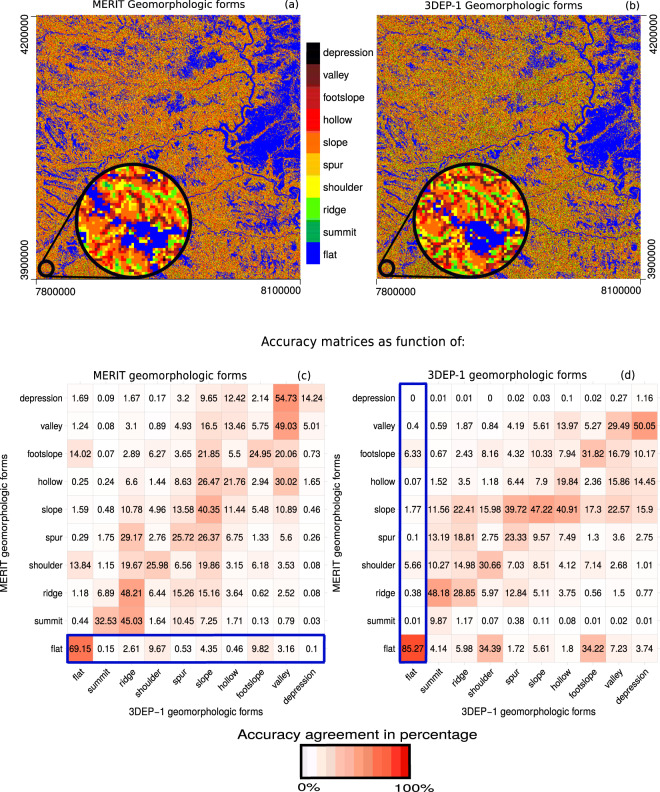
Topographical relief comprises the vertical and horizontal variations of the Earth's terrain and drives processes in geomorphology, biogeography, climatology, hydrology and ecology. Its characterisation and assessment, through geomorphometry and feature extraction, is fundamental to numerous environmental modelling and simulation analyses. We, therefore, developed the Geomorpho90m global dataset comprising of different geomorphometric features derived from the MERIT-Digital Elevation Model (DEM) - the best global, high-resolution DEM available. The fully-standardised 26 geomorphometric variables consist of layers that describe the (i) rate of change across the elevation gradient, using first and second derivatives, (ii) ruggedness, and (iii) geomorphological forms. The Geomorpho90m variables are available at 3 (~90 m) and 7.5 arc-second (~250 m) resolutions under the WGS84 geodetic datum, and 100 m spatial resolution under the Equi7 projection. They are useful for modelling applications in fields such as geomorphology, geology, hydrology, ecology and biogeography.

Fig. 1

Maximum multiscale roughness. Quasi-global representation of the MERIT-derived maximum multiscale roughness (rough-magnitude), computed under Equi7 with a pixel size of 100 m using the computation parameters reported in the Multiscale roughness description. For the purpose of plotting the graphs, the 100 m resolution was aggregated to 1 km (10 × 10 pixels) by calculating the mean. Projection distortion of each Equi7 zone does not allow the merging of zones for a global continuous surface. However, the zones have been positioned adjacent to each other as a mosaic of six projections with gaps in between, to present a quasi-global map. Global visualisation in WGS84 for the other geomorphometric variables can be seen on the Geomorpho90m webpage.

Fig. 2

Projection bias assessment. Graphical representation of the difference in terrain slope calculation due to the effect of using the World Geodetic System 1984 (WGS84) (raster panels right-hand side) compared to the Equi7 projection (raster panels left-hand side). A study area located in the subtropical zone (image centre: longitude −83.26, latitudes 9.05) was used to subset the MERIT-DEM for an area of 500 × 500 grid cells (g). This area has been transposed to a subarctic zone (image centre: longitude −38.19, latitudes 72.80) under the Equi7 projection (a). After having been reprojected to WGS84 (b,h), the variable slope was calculated in the four conditions (c–f), and then reprojected back to Equi7 for comparisons (see blue line-arrows). The scatter plots on the right-hand side shows the WGS84-MERIT slope (d,f) vs. the MERIT slope under the Equi7 projection (c,e), respectively for the subarctic zone (i) and for the subtropical zone (j). The red lines represent the 1:1 relationship and black lines represent a linear model between the two axes. The slope calculated under WGS84 in the subarctic zone is clearly underestimated compared to the one calculated under the Equi7 projection.

Fig. 3

Elevation Deviation Index. Elevation Deviation Index EDI (c) obtained as the ratio of elevation difference (a: 3DEP-1 - MERIT) and elevation standard deviation calculated using a moving window of 5 × 5 pixels of the 3DEP-1 (b). The coordinates reported in a are in Equi7 and expressed in metres. The study area refers to a zone of 18.4 × 20 km, which has a high level of forest cover, and is located in Alberta, Canada, close to Jasper National Park - image centre 118.25°W 53.29°N. The same area is used in the Fig. 4 to assess the geomorphometric variables.

Fig. 4

Normalised difference maps. Normalised difference maps represented as Δ surface, for each geomorphometric variable derived from 3DEP-1 minus MERIT-DEM. To compare the geomorphometric variables under the same scale unit, the difference has been scaled from -1 to 1 (minimum and maximum stretching) keeping the 0 value (no difference) at the 0 position. The bottom plot reports the normalised difference as mean (blue line) and standard deviation values (orange vertical lines) of the maps. The mean and standard deviation plot helps to identify which geomorphometric variables are more sensitive to variation in the DEMs (e.g. high sensitivity for variables derived from slope and aspect). The coordinates u in Equi7 are expressed in metres and refer to a study area of 18.4 × 20 km, which has a high level of forest cover, and is located in Alberta, Canada, close to Jasper National Park - image centre 118.25°W 53.29°N.

Fig. 5

Geomorphological forms maps and confusion matrices. The geomorphological forms have been computed for a study area of 3000 × 3000, 100 m pixels in South Dakota (USA) derived from MERIT (a–c) and 3DEP-1 (b–d), respectively. The confusion matrix values are expressed in percentages of the MERIT-DEM classes, with the sum of vertical values equal to 100 (d); and of the 3DEP-1 classes, with the sum of the horizontal values equal to 100 (c). The sum of the values in the blue boxes is equal to 100, and so on for each row (c) and column (d).

Fig. 6

MERIT-DEM vs LiDAR-DEM. Comparison of MERIT-DEM with the LiDAR DSM and LiDAR DTM for four study areas, represented by their scatter-plots and their relative linear models.

References

1. Pike RJ. Geomorphometry-diversity in quantitative surface analysis. Progress in physical geography. 2000;24:1–20.
1. Florinsky IV. An illustrated introduction to general geomorphometry. Progress in Physical Geography. 2017;41:723–752.
1. Alexander C, Deák B, Heilmeier H. Micro-topography driven vegetation patterns in open mosaic landscapes. Ecological indicators. 2016;60:906–920.
1. Stein A, Kreft H. Terminology and quantification of environmental heterogeneity in species-richness research. Biological Reviews. 2015;90:815–836. - PubMed
1. Amatulli G, et al. A suite of global, cross-scale topographic variables for environmental and biodiversity modeling. Scientific data. 2018;5:180040. - PMC - PubMed