Interpretable multimodal deep learning for real-time pan-tissue pan-disease pathology search on social media

Abstract

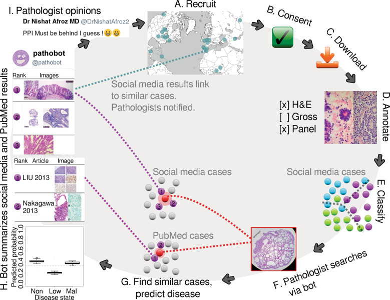
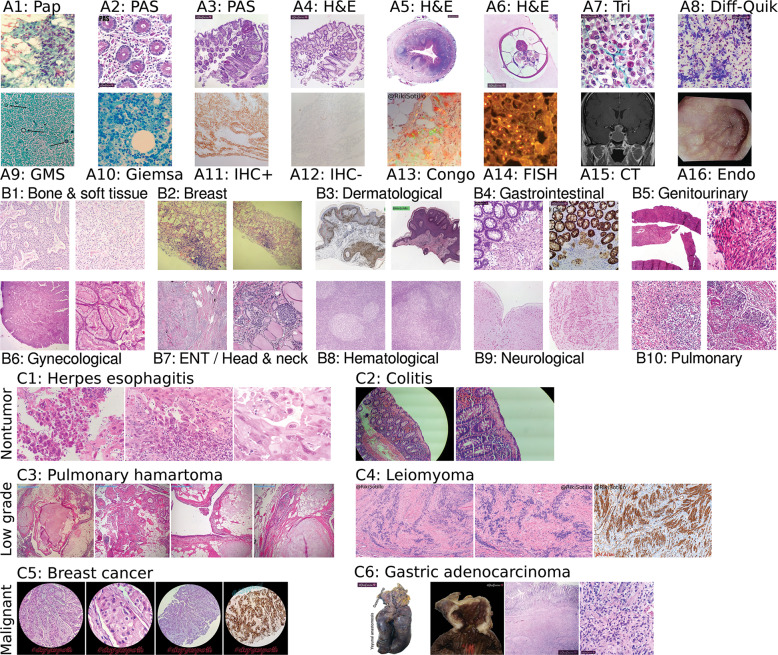
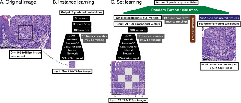
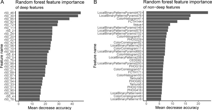
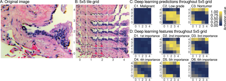
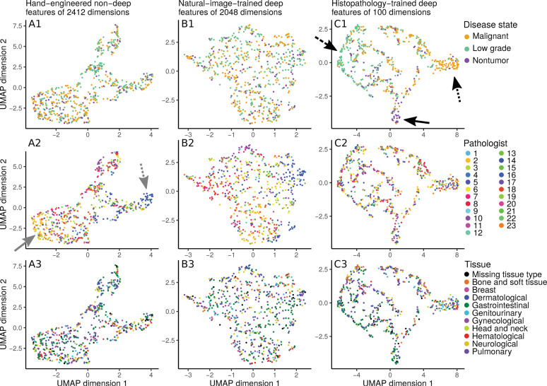
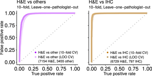
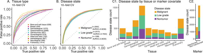
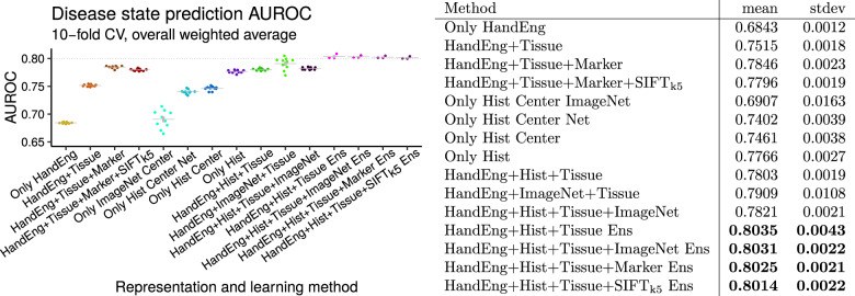
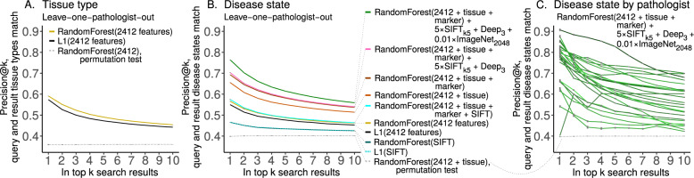
Pathologists are responsible for rapidly providing a diagnosis on critical health issues. Challenging cases benefit from additional opinions of pathologist colleagues. In addition to on-site colleagues, there is an active worldwide community of pathologists on social media for complementary opinions. Such access to pathologists worldwide has the capacity to improve diagnostic accuracy and generate broader consensus on next steps in patient care. From Twitter we curate 13,626 images from 6,351 tweets from 25 pathologists from 13 countries. We supplement the Twitter data with 113,161 images from 1,074,484 PubMed articles. We develop machine learning and deep learning models to (i) accurately identify histopathology stains, (ii) discriminate between tissues, and (iii) differentiate disease states. Area Under Receiver Operating Characteristic (AUROC) is 0.805-0.996 for these tasks. We repurpose the disease classifier to search for similar disease states given an image and clinical covariates. We report precision@k = 1 = 0.7618 ± 0.0018 (chance 0.397 ± 0.004, mean ±stdev ). The classifiers find that texture and tissue are important clinico-visual features of disease. Deep features trained only on natural images (e.g., cats and dogs) substantially improved search performance, while pathology-specific deep features and cell nuclei features further improved search to a lesser extent. We implement a social media bot (@pathobot on Twitter) to use the trained classifiers to aid pathologists in obtaining real-time feedback on challenging cases. If a social media post containing pathology text and images mentions the bot, the bot generates quantitative predictions of disease state (normal/artifact/infection/injury/nontumor, preneoplastic/benign/low-grade-malignant-potential, or malignant) and lists similar cases across social media and PubMed. Our project has become a globally distributed expert system that facilitates pathological diagnosis and brings expertise to underserved regions or hospitals with less expertise in a particular disease. This is the first pan-tissue pan-disease (i.e., from infection to malignancy) method for prediction and search on social media, and the first pathology study prospectively tested in public on social media. We will share data through http://pathobotology.org . We expect our project to cultivate a more connected world of physicians and improve patient care worldwide.

Fig. 1. Graphical summary.

Pathologists are recruited worldwide (A). If a pathologist consents to having their images used (B), we download those images (C) and manually annotate them (D). Next, we train a Random Forest classifier to predict image characteristics, e.g., disease state (E). This classifier is used to predict disease and search. If a pathologist posts a case to social media and mentions @pathobot (F), our bot will use the post’s text and images to find similar cases on social media and PubMed (G). The bot then posts summaries and notifies pathologists with similar cases (H). Pathologists discuss the results (I), and some also decide to share their cases with us, initiating the cycle again (A). “Procedure overview” in the supplement explains further (Section S5.4).

Fig. 2. Technique, tissue, and disease diversity.

Panel set A shows diverse techniques in our data. Initials indicate author owning image. A1 RSS: papanicolaou stain. A2 LGP: periodic acid–Schiff (PAS) stain, glycogen in pink. A3 LGP: PAS stain, lower magnification. A4 LGP: H&E stain c.f. Panel A3. A5 LGP: H&E stain, human appendix, including parasite Enterobius vermicularis (c.f. Fig. S2). A6 LGP: Higher magnification E. vermicularis c.f. Panel A5. A7 LGP: Gömöri trichrome, collagen in green. A8 LGP: Diff-quik stain, for cytology. A9 RSS: GMS stain (“Intra-stain diversity” in supplement details variants, Section S5.3.1), fungi black. A10 MPP: Giemsa stain. A11 AM: immunohistochemistry (IHC) stain, positive result. A12 AM: IHC stain, negative result. A13 RSS: Congo red, polarized light, plaques showing green birefringence. A14 MPP: fluorescence in situ hybridization (FISH) indicating breast cancer Her2 heterogeneity. A15 SY: head computed tomography (CT) scan. A16 LGP: esophageal endoscopy. In panel set B we show differing morphologies for all ten histopathological tissue types on Twitter. B1 CS: bone and soft tissue. We include cardiac here. B2 KH: breast. B3 RSS: dermatological. B4 LGP: gastrointestinal. B5 OOF: genitourinary. B6 MPP: gynecological. B7 BX: otorhinolaryngological a.k.a. head and neck. We include ocular, oral, and endocrine here. B8 CS: hematological, e.g., lymph node. B9 SY: neurological. B10 SM: pulmonary. In panel set C we show the three disease states we use: nontumor, low grade, and malignant. C1 MPP: nontumor disease, i.e., herpes esophagitis with Cowdry A inclusions. C2 KH: nontumor disease, i.e., collagenous colitis showing thickened irregular subepithelial collagen table with entrapped fibroblasts, vessels, and inflammatory cells. C3 AM: low grade, i.e., pulmonary hamartoma showing entrapped clefts lined by respiratory epithelium. C4 RSS: low grade, i.e., leiomyoma showing nuclear palisading. We show IHC completeness but it is not included for machine learning. C5 BDS: malignant, i.e., breast cancer with apocrine differentiation. C6 LGP: malignant, i.e., relapsed gastric adenocarcinoma with diffuse growth throughout the anastomosis and colon. Gross sections (e.g., Fig. S3) shown for completeness but not used.

Fig. 3. Deep learning methods summary.

A An overall input image may be of any size, but must be at least 512 × 512 pixels (px). B We use a ResNet-50 [29] deep convolutional neural network to learn to predict disease state (nontumor, low grade, or malignant) on the basis of a small 224 × 224 px patch. This small size is required to fit the ResNet-50 and image batches in limited GPU memory. C For set learning, this network transforms each of the 21 patches sampled evenly from the image in a grid to a 100-dimensional vector. These 21 patches span the overall input image entirely. For instance, if the overall input image is especially wide, the 21 patches will overlap less in the X dimension. The ResNet-50 converts these 21 patches to 21 vectors. These 21 vectors are summed to represent the overall image, regardless of the original image’s size, which may vary. This sum vector is concatenated with tissue covariates (which may be missing for some images), marker mention covariate, and hand-engineered features. A Random Forest then learns to predict disease state on this concatenation that encodes (i) task-agnostic hand-engineered features (Fig. S9) near the image center, (ii) task-specific features from deep learning throughout the image, (iii) whether IHC or other markers were mentioned for this case, and (iv) optionally tissue type. Other machine learning tasks, e.g., histology stain prediction and tissue type prediction, were simpler. For simpler tasks, we used only the Random Forest and 2412 hand-engineered features, without deep learning.

Fig. 4. Random Forest feature importance for prioritizing deep features, when non-deep, deep, and clinical features are used together for learning.

We use the mean decrease in accuracy to measure Random Forest feature importance. To do this, first, a Random Forest is trained on task-agnostic hand-engineered features (e.g., color histograms), task-specific deep features (i.e., from the ResNet-50), and the tissue type covariate that may be missing for some patients. Second, to measure the importance of a feature, we randomly permute/shuffle the feature’s values, then report the Random Forest’s decrease in accuracy. When shuffling a feature’s values this way, more important features result in a greater decrease in accuracy, because accurate prediction relies on these features more. We show the most important features at the top of these plots, in decreasing order of importance, for deep features (A) and non-deep features (B). The most important deep feature is “r50_46”, which is the output of neuron 47 of 100 (first neuron is 0, last is 99), in the 100-neuron layer we append to the ResNet-50. Thus of all 100 deep features, r50_46 may be prioritized first for interpretation. Of non-deep features, the most important features include Local Binary Patterns Pyramid (LBPP), color histograms, and “tissue” (the tissue type covariate). LBPP and color histograms are visual features, while tissue type is a clinical covariate. LBPP are pyramid-based grayscale texture features that are scale-invariant and color-invariant. LBPP features may be important because we neither control the magnification a pathologist uses for a pathology photo, nor do we control. staining protocol. For a before-and-after training comparison that may suggest the histopathology-trained deep features represent edges, colors, and tissue type rather than texture, we also analyze feature importance of only natural-image-trained ImageNet₂₀₄₈ deep features in conjunction with hand-engineered features (Fig. S10). “Marker mention and SIFT features excluded from Random Forest feature importance analysis” discusses other details in the supplement (Section S5.10.2).

Fig. 5. Interpretable spatial distribution of deep learning predictions and features.

A An example image for deep learning prediction interpretation, specifically a pulmonary vein lined by enlarged hyperplastic cells, which we consider to be low-grade disease state. Case provided by YR. B The image is tiled into a 5 × 5 grid of overlapping 224 × 224 px image patches. For heatmaps, we use the same 5 × 5 grid as in Fig. 1C bottom left, imputing with the median of the four nearest neighbors for 4 of 25 grid tiles. C We show deep learning predictions for disease state of image patches. At left throughout the image, predictions have a weak activation value of 0 for malignant, so these patches are not predicted to be malignant. At middle the centermost patches have a strong activation value of 1, so these patches are predicted to be low grade. This spatial localization highlights the hyperplastic cells as low grade. At right the remaining normal tissue and background patches are predicted to be nontumor disease state. Due to our use of softmax, we note that the sum of malignant, low-grade, and nontumor prediction activation values for a patch equals 1, like probabilities sum to 1, but our predictions are not Gaussian-distributed probabilities. D We apply the same heatmap approach to interpret our ResNet-50 deep features as well. D1 the most important deep feature corresponds to the majority class prediction, i.e., C1, malignant. D2 The second most important deep feature corresponds to prediction of the second most abundant class, i.e., C2, low grade. D3 The third most important deep feature corresponds to prediction of the third most abundant class, i.e., C3, nontumor. The fourth (D4) and fifth (D5) most important features also correspond to nontumor. D6 The sixth most important deep feature does not have a clear correspondence when we interpret the deep learning for this case and other cases (Fig. S11), so we stop interpretation here. As expected, we did not find ImageNet₂₀₄₈ features to be interpretable from heatmaps, because these are not trained on histpathology (Fig. S11A5).

Fig. 6. Disease state clusters based on hand-engineered, natural-image-trained deep features, or histopathology-trained deep features.

To determine which features meaningfully group patients together, we apply the UMAP [34] clustering algorithm on a held-out set of 10% of our disease state data. Each dot represents an image from a patient case. In general, two dots close together means these two images have similar features. Columns indicate the features used for clustering: hand-engineered features (at left column), only-image-trained ImageNet₂₀₄₈ deep features (at middle column), or histopathology-trained deep features (at right column). Rows indicate how dots are colored: by disease state (at top row), by contributing pathologist (at middle row), or by tissue type (at bottom row). For hand-engineered features, regardless of whether patient cases are labeled by disease state (A1), pathologist (A2), or tissue type (A3), there is no strong clustering of like-labeled cases. Similarly, for only natural-image-trained ImageNet₂₀₄₈ deep features, there is no obvious clustering by disease state (B1), pathologist (B2), or tissue type (B3). However, for histopathology-trained deep features, patient cases cluster by disease state (C1), with separation of malignant (at dotted arrow), low grade (at dashed arrow), and nontumor (at solid arrow). There is no clear clustering by pathologist (C2) or tissue type (C3). The main text notes that hand-engineered features may vaguely group by pathologist (A2, pathologists 2 and 16 at solid and dotted arrows).

Fig. 7. H&E performance.

Predicting if an image is acceptable H&E human tissue or not (at left), or if image is H&E rather than IHC (at right). Ten replicates of ten-fold cross-validation (tenfold) and leave-one-pathologist-out cross-validation (LOO) had similarly strong performance. This suggests the classifier may generalize well to other datasets. We use the “H&E vs. others” classifier to find H&E images in PubMed. Shown replicate AUROC for H&E vs. others is 0.9735 for tenfold (ten replicates of tenfold has mean ± stdev of 0.9746 ± 0.0043) and 0.9549 for LOO (ten replicates 0.9547 ± 0.0002), while H&E vs. IHC is 0.9967 for tenfold (ten replicates 0.9977 ± 0.0017) and 0.9907 for LOO (ten replicates 0.9954 ± 0.0004). For this and other figures, we show the first replicate.

Fig. 8. Ten tissue type and three disease state prediction performance and counts.

A Classifier performance for predicting histopathology tissue type (ten types, 8331 images). B Classifier performance for predicting disease state (three disease states; 6549 images). Overall AUROC is the weighted average of AUROC for each class, weighted by the instance count in the class. These panels (A, B) show AUROC (with ten-fold cross-validation) for the chosen classifier. Random Forest AUROC for tissue type prediction is 0.8133 (AUROC for the ten replicates: mean ± stdev of 0.8134 ± 0.0007). AUROC is 0.8085 for an ensemble of our deep-learning-Random-Forest hybrid classifiers for disease state prediction (AUROC for the ten replicates: mean ± stdev of 0.8035 ± 0.0043). C1 Disease state counts per tissue type. The proportion of nontumor vs. low-grade vs. malignant disease states varies as a function of tissue type. For example, dermatological tissue images on social media are most often low grade, but malignancy is most common for genitourinary images. C2 Disease state counts as a function of whether a marker test (e.g., IHC, FISH) was mentioned (˜25% of cases) or not. IHC is the most common marker discussed and is typically, but not necessarily, used to subtype malignancies.

Fig. 9. Disease state prediction performance for machine learning methods..

For deep learning we use a ResNet-50. For shallow learning we use a Random Forest. We train a Random Forest on deep features (and other features), to combine deep and shallow learning (Fig. 3C top). Error bars indicate standard error of the mean. Points indicate replicates. Gray lines indicate means. Performance increases markedly when including tissue type covariate for learning (even though tissue type is missing for some patients), when using deep learning to integrate information throughout entire image rather than only the center crop, and when using an ensemble of classifiers. Performance exceeds AUROC of 0.8 (at right). We conclude method xii (“HandEng + Hist + Tissue Ens”) is the best we tested for disease state prediction, because no other method performs significantly better and no other simpler method performs similarly. Methods are, from left to right, (i) Random Forest with 2412 hand-engineered features alone for 512 × 512 px scaled and cropped center patch, (ii) Random Forest with tissue covariates, (iii) Random Forest with tissue and marker covariates, (iv) method iii additionally with SIFT_k5 features for Random Forest, (v) only natural-image-trained ResNet-50 at same scale as method i with center 224 × 224 px center patch and prediction from a Random Forest trained on 2048 features from the ResNet-50 (Fig. 3), (vi) histopathology-trained ResNet-50 at same scale as method i with center 224 × 224 px center patch and prediction from top three neurons (Fig. 3B top), (vii) histopathology-trained ResNet-50 with Random Forest trained on 100 features from 224 × 224 px center patch per method vi, (viii) histopathology-trained ResNet-50 features at 21 locations throughout image summed and Random Forest learning on this 100-dimensional set representation with 2412 hand-engineered features, (ix) method viii with tissue covariates for histopathology-trained ResNet-50 and 2412 hand-engineered features for Random Forest learning (i.e., Fig. 3C sans marker information), (x) method ix with an only natural-image-trained ResNet-50 instead of a histopathology-trained ResNet-50 for Random Forest learning, (xi) method ix with both an only natural-image-trained ResNet-50 and a histopathology-trained ResNet-50 for Random Forest learning, (xii) method ix with an ensemble of three Random Forest classifiers such that each classifier considers an independent histopathology-trained ResNet-50 feature vector in addition to 2412 hand-engineered features and tissue covariate, (xiii) method xii where each Random Forest classifier in ensemble additionally considers only natural-image-trained ResNet-50 features, (xiv) method xii where each Random Forest classifier in ensemble additionally considers the marker mention covariate (i.e., this is an ensemble of three classifiers where Fig. 3C is one of the three classifiers), (xv) method xii where each Random Forest in ensemble additionally considers SIFT_k5 features for learning.

Fig. 10. Case similarity search performance.

We report search performance as precision@k for leave-one-pathologist-out cross-validation for (A) tissue and (B) disease state. We note search based on SIFT features performs better than chance, but worse than all alternatives we tried. Marker mention information improves search slightly, and we suspect cases that mention markers may be more relevant search results if a query case also mentions markers. SIFT_k5 and histopathology-trained Deep₃ features improve performance even less, but only natural-image-trained ImageNet₂₀₄₈ deep features increase performance substantially (Table S1). (C) We show per-pathologist variability in search, with outliers for both strong and weak performance. Random chance is dashed gray line. In our testing, performance for every pathologist is always above chance, which may suggest performance will be above chance for patient cases from other pathologists. We suspect variability in staining protocol, variability in photography, and variability in per-pathologist shared case diagnosis difficulty may underlie this search performance variability. The pathologist where precision@k = 1 is lowest shared five images total for the disease prediction task, and these images are of a rare tissue type. Table S2 shows per-pathologist performance statistics.

References

1. Transforming Our World: The 2030 Agenda for Sustainable Development. In Rosa W, editor. A New Era in Global Health. Springer Publishing Company. ISBN 978-0-8261-9011-6 978-0-8261-9012-3. 2017:545-6.
1. Nix J, Gardner J, Costa F, Soares A, Rodriguez F, Moore B, et al. Neuropathology education using social media. J Neuropathol Exp Neurol. 2018;77:454–60. doi: 10.1093/jnen/nly025. - DOI - PubMed
1. Crane G, Gardner J. Pathology image-sharing on social media: recommendations for protecting privacy while motivating education. AMA J Ethics. 2016;18:817–25. doi: 10.1001/journalofethics.2016.18.8.stas1-1608. - DOI - PubMed
1. Dirilenoglu F, Önal B. A welcoming guide to social media for cytopathologists: tips, tricks, and the best practices of social cytopathology. CytoJournal. 2019;16:4. doi: 10.4103/cytojournal.cytojournal_1_18. - DOI - PMC - PubMed
1. Gardner J, Allen T. Keep calm and tweet on: legal and ethical considerations for pathologists using social media. Arch Pathol Lab Med. 2018;143:75–80. doi: 10.5858/arpa.2018-0313-SA. - DOI - PubMed
Publication types
LinkOut - more resources