A map of object space in primate inferotemporal cortex

Abstract

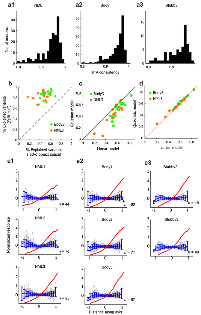
The inferotemporal (IT) cortex is responsible for object recognition, but it is unclear how the representation of visual objects is organized in this part of the brain. Areas that are selective for categories such as faces, bodies, and scenes have been found^1-5, but large parts of IT cortex lack any known specialization, raising the question of what general principle governs IT organization. Here we used functional MRI, microstimulation, electrophysiology, and deep networks to investigate the organization of macaque IT cortex. We built a low-dimensional object space to describe general objects using a feedforward deep neural network trained on object classification⁶. Responses of IT cells to a large set of objects revealed that single IT cells project incoming objects onto specific axes of this space. Anatomically, cells were clustered into four networks according to the first two components of their preferred axes, forming a map of object space. This map was repeated across three hierarchical stages of increasing view invariance, and cells that comprised these maps collectively harboured sufficient coding capacity to approximately reconstruct objects. These results provide a unified picture of IT organization in which category-selective regions are part of a coarse map of object space whose dimensions can be extracted from a deep network.

Extended Data Figure 1.. Time courses from NML1-3 during microstimulation of NML2.

a. Sagittal (top) and coronal (bottom) slices showing activation to microstimulation of NML2. Dark track shows electrode targeting NML2. b. Time courses of microstimulation together with fMRI response from each of the three patches of the NML network.

Extended Data Figure 2.. Stimuli used in electrophysiological recordings.

a. 51 objects from 6 categories were shown to monkeys. b. 24 views for one example object, resulting from rotations in the x-z plane (abscissa) combined with rotations in the y-z plane (ordinate). c. A line segment parametrically varied along three dimensions was used to test the hypothesis that cells in the NML network are selective for aspect ratio: 4 aspect ratio levels × 13 curvature levels × 12 orientation levels. d. 36 example object images from an image set containing 1593 images.

Extended Data Figure 3.. Additional neuronal response properties from different patches.

a1. Average responses to 51 objects across all cells from patch NML2 are plotted against those from patch NML1. The response to each object was defined as the average response across 24 views and across all cells recorded from a given patch. b1. Same as (a1) for NML3 against NML2. (c1) Same as (a1) for NML3 against NML1. (a2, b2, c2) Same as (a1, b1, c1) for three patches of the body network. a3. Same as (a1) for Stubby3 against Stubby2. d. Similarity matrix showing the Pearson correlation values (r) between the average responses to 51 objects from 9 patches across 4 networks. e. Left: cumulative distributions of view-invariant identity correlations for cells in the three patches of the NML network. Right: same as left, for cells in the three patches of the body network. For each cell, the view-invariant identity correlation was computed as the average across all pairs of views of the correlation between response vectors to the 51 objects at a pair of distinct views. The distribution of view-invariant identity correlations was significantly different between NML1 and NML2 (t-test two-tailed, p < 0.005, t(118) = 2.96), NML2 and NML3 (t-test two-tailed, p < 0.005, t( 169) = 2.9), Body1 and Body2 (t-test two-tailed, p < 0.0001, t(131) = 6.4), and Body2 and Body3 (t-test two-tailed, p < 0.05, t(126) = 2.04). * means p < 0.05, ** means p < 0.01. (f1) Time course of view-invariant object identity selectivity for the three patches in the NML network, computed using responses to 11 objects at 24 views and a 50-ms sliding response window (solid lines). As a control, time courses of correlations between responses to different objects across different views were also computed (dashed lines) (see Methods). f2. Same as (f1) for body network. (f3) Same as (f1) for stubby network. g. Top: Average responses to each image across all cells recorded from each patch are plotted against the logarithm of aspect ratio of the object in each image (see Methods). Pearson r values are indicated in each plot (all p < 10⁻¹⁰). The rightmost column shows results with cells from all three patches grouped together. Bottom: Same as top, with responses to each object averaged across 24 views, and associated aspect ratios also averaged. The rightmost column shows results with cells from all three patches grouped together.

Extended Data Figure 4.. Building an object space using a deep network.

a. A diagram illustrating the structure of AlexNet. Five convolution layers are followed by three fully connected layers. The number of units in each layer is indicated below each layer. b. Images with extreme values (highest: red, lowest: blue) of PC1 and PC2 are shown. c. The cumulative explained variance of responses of units in fc6 by 100 PCs; 50 dimensions explain 85% variance. d. Images in the 1593 image set with extreme values (highest: red, lowest: blue) of PC1 and PC2 built by the 1593 image set after affine transform (see Methods). Preferred features are generally consistent with those computed using the original image set shown in (b). However, PC2 no longer clearly corresponds to an animate-inanimate axis; instead, it corresponds to curved versus rectilinear shapes. e. Distributions showing the canonical correlation value between the first two PCs obtained by the 1224 image set and first two PCs built by other sets of images (1224 randomly selected non-background object images, left: PC1, right: PC2; see Methods for details). The red triangles indicate the average of the distributions. f. 19,300 object images were passed through AlexNet and PC1-PC2 space was built with PCA. Then we projected 1224 images on this PC1-PC2 space. The top 100 images for each network are indicated by colored dots (compare Fig. 4b). (g) Decoding accuracy for 40 images using object spaces built by responses of different layers of AlexNet (computed as in Extended Data Fig. 11d). There are multiple points for each layer because we performed PCA before and after pooling, activation, and normalization functions. Layer fc6 showed highest decoding accuracy, motivating our use of the object space generated by this layer throughout the paper. h. To compare IT clustering determined by AlexNet with that by other deep network architectures, we first determined the layer of each network giving best decoding accuracy, as in (g). The bar plot shows decoding accuracy for 40 images in the 9 different networks using the best-performing layer for each network. i. Canonical correlation values between the first two PCs obtained by Alexnet and first two PCs built by 8 other deep-learning networks (labelled as 2-9). The layer of each network yielding highest decoding accuracy for 40 images was used for this analysis. The name of each network and layer name can be found in (j). j. Same as Fig. 4b using PC1 and PC2 computed from 8 other networks.

Extended Data Figure 5.. Neurons across IT perform axis coding.

a1. The distribution of consistency of preferred axis for cells in the NML network (see Methods). a2. Same as (a1) for the body network. a3. Same as (a1) for the stubby network. (b) Different trials of responses to the stimuli were randomly split into two halves, and the average response across half of the trials was used to predict that of the other half. Percentage variances explained, after Spearman-Brown correction (mean = 87.8%), are plotted against that of the axis model (mean = 49.1%). Mean explainable variance for 29 cells was 55.9%. c. Percentage variances explained by a Gaussian model are plotted against that of the axis model. d. Percentage variances explained by a quadratic model are plotted against that of the axis model. Inspection of coefficients of the quadratic model revealed a negligible quadratic term (mean ratio of 2^nd-order coefficients/1^st-order coefficient = 0.028). (e1) Top: The red line shows the average modulation along the preferred axis across the population of NML1 cells. The gray lines show, for each cell in NML1, the modulation along the single axis orthogonal to the preferred axis the in 50-d objects space that accounts for the most variability. The blue line and error bars represent the mean and SD of the gray lines. Middle, bottom: analogous plots for NML2 and NML3. e2. Same as (e1) for the three body patches. (e3) Same as (e1) for the two stubby patches.

Extended Data Figure 6.. Similar functional organization is observed using a different stimulus set.

a. Projection of preferred axes onto PC1 versus PC2 for all neurons recorded using two different stimulus sets (left: 1593 images from freepngs image set, right: the original 1224 images consisting of 51 objects × 24 views). The PC1-PC2 space for both plots was computed using the 1224 images. Different colors encode neurons from different networks. b. Top 21 preferred stimuli based on average responses from the neurons recorded in three networks to the two different image sets. (c1) Four classes of silhouette images projecting strongly on the four quadrants of object space. c2. Coronal slices from posterior, middle, and anterior IT of monkeys M2 and M3 showing the spatial arrangement of the four networks revealed with silhouette images of (c1) in an experiment analogous to that in Fig. 4a. (d1) Four classes of “fake object” images projecting strongly on the four quadrants of object space. Note fake objects projecting onto the face quadrant no longer resembled real faces. d2. Same as (c2) with fake object images of (d1). (e1) Four example stimuli generated by deep dream techniques projecting strongly on the four quadrants of object space. e2. Same as (c2) with deep dream images of (e1). The results in (c-e) support the idea that IT is organized according to the first two axes of object space rather than low-level features, semantic meaning, or image organization.

Extended Data Figure 7.. Response time courses from the four IT networks spanning object space.

Time courses were averaged across two monkeys. To avoid selection bias, odd runs were used to identity regions of interest, and even runs were used to compute average time courses from these regions.

Extended Data Figure 8.. Searching for substructure within patches.

a. Axial view of the Stubby2 patch, together with projections of three recording sites. b. Mean responses to 51 objects from neurons grouped by recording sites shown in (a) (same format as Fig. 2a1). c. Axial view of the Stubby3 patch, together with projections of two recording sites. d. Mean responses to 51 objects from neurons grouped by recording sites shown in (c). e. Projection of preferred axis onto PC1-PC space for neurons recorded from different sites within the Stubby2 patch. There is no clear separation between neurons from the three sites in PC1-PC2 space. The gray dots represent all other neurons across the four networks. f. Same as (e) for cells recorded from two sites in the Stubby3 patch. g1. Projection of preferred axes onto PC1-PC2 space for all recorded neurons. Different colors encode neurons from different networks. g2. Same as (g1), but the color represents the cluster that the neuron belongs to. Clusters were determined by k-means analysis, with number of clusters set to 4, and distance between neurons defined by the correlation between preferred axes in the 50-d object space (see Methods). Comparison of (g1) and (g2) reveals highly similarity between the anatomical clustering of IT networks and the functional clustering determined by k-means analysis. g3. Calinski-Harabasz criterion values were plotted against the number of clusters for k-means analysis performed with different number of clusters (see Methods). The optimal cluster number is 4. h1. Same as (g1) for projection of preferred axes onto PC3 versus PC4. (h2) Same as (h1), but the color represents the cluster that the neurons belongs to. Clusters were determined by k-means analysis, with number of clusters set to 4, and distance between neurons defined by the correlation between preferred axes in the 48-d object space obtained by removing the first two dimensions. The difference between (h1) and (h2) suggests there is no anatomical clustering for dimensions beyond the first two PCs. (h3) Same as (g3), with k-means analysis in the 48-d object space. By the Calinski-Harabasz criterion, there is no functional clustering for higher dimensions beyond the first two.

Extended Data Figure 9.. The object space model parsimoniously explains previous accounts of IT organization.

a1. The object images used in are projected onto object PC1-PC2 space (computed as in Fig. 4b, by first passing each image through AlexNet). A clear gradient from big (red) to small (blue) objects is seen. a2. Same as (a1), for the inanimate objects (big and small) used in . a3. Same as (a1), for the original object images used in . a4. Same as (a1) for the texform images used in . (b2, b3, b4) Projection of animate and inanimate images from original object images (b2, b3) and texforms (b4). c. Left: colored dots depict projection of stimuli from the four conditions used in . Right: example stimuli (blue: small object-like, cyan: large object-like, red: landscape-like, magenta: cave-like). d. Left: gray dots depict 1224 stimuli projected onto object PC1-PC2 space; colored dots depict projection of stimuli from the four blocks of the curvature localizer used in . Right: example stimuli from the four blocks of the curvature localizer (blue: real-world round shapes, cyan: computer-generated 3D sphere arrays, red: real-world rectilinear shapes, magenta: computer-generated 3D pyramid arrays). e. Images of English and Chinese words are projected onto object PC1-PC2 space (black diamonds), superimposed on the plot from Fig. 4b. They are grouped into a small region, consistent with their modular representation by the VWFA.

Extended Data Figure 10.. Object space dimensions are a better descriptor of response selectivity in the body patch than category labels.

a. Four classes of stimuli: body stimuli projecting strongly onto body quadrant of object space (bright red), body stimuli projecting weakly onto body quadrant of object space (dark red), non-body stimuli projecting equally strongly as (2) onto body quadrant of object space (dark blue), and non-body stimuli projecting negatively onto body quadrant of object space (bright blue). b. Predicted response of the body patch to each image from the four stimulus conditions in (a), computed by projecting the object space representation of each image onto the preferred axis of the body patch (determined from the average response of body patch neurons to the 1224 stimuli). c. Left: fMRI response time course from the body patches to the four stimulus conditions in (a). Center: Mean normalized single-unit responses from neurons in body1 patch to the four stimulus conditions. The error band represents the SE across different neurons. Right: Mean local field potential (LFP) from body1 patch to the four stimulus conditions. The error band represents the SE across different recording sites.

Extended Data Figure 11.. Object decoding and recovery of images by searching a large auxiliary object database.

a. Schematic illustrating the decoding model. To construct and test the model, we used responses of m recorded cells to n images. Population responses to images from all but one object were used to determine the transformation from responses to feature values by linear regression, and then the feature values of the remaining object were predicted (for each of 24 views). b. Model predictions are plotted against actual feature values for the first PC of object space. c. Percentage explained variances for all 50 dimensions using linear regression based on responses of four different neural populations: 215 NML cells (yellow); 190 body cells (green); 67 stubby cells (magenta); 482 combined cells (black). d. Decoding accuracy as a function of number of object images randomly drawn from the stimulus set for the same four neural populations as in (c). Dashed line indicates chance performance. e. Decoding accuracy for 40 images plotted against different numbers of cells randomly drawn from same four populations as (c). f. Decoding accuracy for 40 images plotted as a function of the numbers of PCs used to parametrize object images. g. Example reconstructed images from the three groups defined in (h) are shown. In each pair, the original image is shown on the left, and image reconstructed using neural data is shown on the right. h. The distribution of normalized distances between predicted and reconstructed feature vectors. The normalized distance takes account of the fact that the object images used for reconstruction did not include any of the object images shown to the monkey, setting a limit on how good the reconstruction can be (see Methods). A normalized distance of 1 means that the reconstruction has found the best solution possible. Images were sorted into three groups based on the normalized distance. i. Distribution of specialization indices SI_ij across objects for the NML (left), body (center) and stubby (right) networks (see Supplementary Information). Example objects for each network with SI_ij ~1 are shown. Red bars: objects with SI_ij significantly greater than 0 (t-test two-tailed, p<0.01).

Fig. 1:. Microstimulation reveals a new anatomical network in IT cortex.

a, Stimulus contrasts used to identify known networks in IT (see Methods), b, Inflated brain (right hemisphere) for monkey M1 showing known IT networks mapped in this animal. Regions activated by microstimulation of NML2 are shown in yellow. All activation maps shown at a threshold of P < 10⁻³ not corrected for multiple comparisons. Yellow and magenta outlines indicate the boundaries of TE and TEO, respectively.

Fig. 2:. Distinct object preferences among four different networks in IT cortex.

a–d, Top, responses of cells to 51 objects from six different categories. Responses to each object were averaged across 24 views. Cells were recorded in three patches (NML1, NML2 and NML3) from the NML network (a); in three patches of the body network (b); in patch ML of the face network (c); and in two patches of the stubby network (d). Middle, blue charts show average responses to each object in each network. Numbers indicate the five most-preferred objects. Bottom, five most-preferred (top row) and least-preferred (bottom row) objects for each network, based on averaged responses; images 1 to 5 are shown from left to right, e, Coronal slices containing NML1, NML2, and NML3 from monkeys M1, M2, M3, and M4 showing difference in activation in response to the five most-preferred versus five least-preferred objects determined from electrophysiology in the NML network of monkey M1. In M1, the microsimulation result is also shown as a cyan overlay with threshold P < 10⁻³, uncorrected. Inset numbers indicate AP coordinate relative to interaural 031. f, Responses of cells from patches NML2 and NML3 of the NML network to a line segment that varied in aspect ratio, curvature, and orientation. Responses are averaged across orientation, and curvature runs from low to high from left to right for each aspect ratio. Aspect ratio accounts for 22.8% of response variance on average across cells, curvature for 5.6% of variance, and orientation for 3.5% of variance.

Fig. 3:. Each network contains a hierarchy of increasingly view-invariant nodes, and single cells in each node show ramp-shaped tuning.

a, Population similarity matrices in the three patches of the NML network (top), three patches of the body network (middle) and two patches of the stubby network (bottom) pooled across monkeys M1 and M2. An 88 × 88 matrix of correlation coefficients was computed from responses of cells in each patch to 88 stimuli (8 views × top 11 preferred objects). b, Responses from three example cells recorded in NML3 (top), the body network (middle) and the stubby network (bottom) to 51 objects at 24 views. Four different views of the most preferred object are shown below each response matrix. c, Responses of neurons recorded from patches in the NML network (top), the body network (middle) and the stubby network (bottom) as a function of distance along the preferred axis. The abscissa is rescaled so that the range [−1,1] covers 95% of the stimuli. Half the stimulus trials were used to compute the preferred axis for each cell, and held-out data were used to plot the responses shown.

Fig. 4:. A map of object space revealed by fMRI.

a, A schematic plot showing the map of objects generated by the first two PCs of object space. The stimuli in the rectangular boxes were used for mapping the four networks shown in c, d using fMRI. b, All the stimuli used in the electrophysiology experiments (Extended Data Fig. 2a, b) projected onto the first two dimensions of object space (grey circles). For each network, the top 100 preferred images are marked (body network: green, face network: blue, stubby network: magenta, NMF network: orange). Numbers in parentheses indicate the number of neurons recorded from each network. c, Coronal slices from posterior, middle, and anterior IT of monkeys M3 and M4 showing the spatial arrangement of the four networks (maps thresholded at P < 10⁻³, uncorrected). Here, the networks were computed using responses to the stimuli in a. d, As in c, showing the four networks in monkeys M3 and M4 overlaid on a flat map of the left hemisphere. e, Left, spatial profiles of the four patches along the cortical surface within posterior IT for data from two hemispheres of four animals. The y-axis shows the nonnalized significance level for each comparison of each voxel, and the x-axis shows the position of the voxel on the cortex (see Methods). Right, anatomical locations of the peak responses plotted against the sequence of quadrants in object space, f, g, As in e for voxels from middle IT (f) and anterior IT (g).

Fig. 5:. Reconstructing objects using neuronal responses from the IT object-topic map.

a, Reconstructions using 482 cells from NMF, body, stubby, and face networks. Example reconstructed images from the three groups defined in b are shown. Each row (group) of four images shows from left to right: 1, the original image; 2, the reconstructed image using the fc6 response pattern to the original image; 3, the reconstructed image using the fc6 response pattern projected onto the 50D object space; and 4, the reconstructed image based on neuronal data. b, Distribution of nomalized distances between reconstructed feature vectors and best-possible reconstmcted feature vectors (see Methods).

References

1. Kanwisher N, McDermott J & Chun MM The fusiform face area: a module in human extrastriate cortex specialized for face perception. Journal of neuroscience 17, 4302–4311 (1997). - PMC - PubMed
1. Tsao DY, Freiwald WA, Knutsen TA, Mandeville JB & Tootell RB Faces and objects in macaque cerebral cortex. Nature neuroscience 6, 989 (2003). - PMC - PubMed
1. Downing PE, Jiang Y, Shuman M & Kanwisher N A cortical area selective for visual processing of the human body. Science 293, 2470–2473 (2001). - PubMed
1. Popivanov ID, Jastorff J, Vanduffel W & Vogels R Heterogeneous single-unit selectivity in an fMRI-defined body-selective patch. Journal of Neuroscience 34, 95–111 (2014). - PMC - PubMed
1. Kornblith S, Cheng X, Ohayon S & Tsao DY A network for scene processing in the macaque temporal lobe. Neuron 79, 766–781 (2013). - PMC - PubMed
Publication types