Confound modelling in UK Biobank brain imaging

Abstract

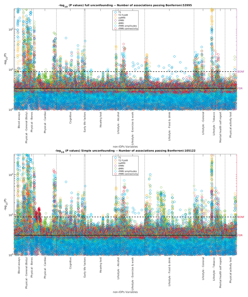
Dealing with confounds is an essential step in large cohort studies to address problems such as unexplained variance and spurious correlations. UK Biobank is a powerful resource for studying associations between imaging and non-imaging measures such as lifestyle factors and health outcomes, in part because of the large subject numbers. However, the resulting high statistical power also raises the sensitivity to confound effects, which therefore have to be carefully considered. In this work we describe a set of possible confounds (including non-linear effects and interactions that researchers may wish to consider for their studies using such data). We include descriptions of how we can estimate the confounds, and study the extent to which each of these confounds affects the data, and the spurious correlations that may arise if they are not controlled. Finally, we discuss several issues that future studies should consider when dealing with confounds.

Keywords: Big data imaging; Confounds; Data modelling; Epidemiological studies; Image analysis; Machine learning; Multi-modal data integration; Statistica l modelling.

Fig. 1

Matrix showing the percentage of variance of each group of confounds explained by each other group. Each row and column represents one group of confounds. These groups can be organised into families: 1: Subject-specific confounds; 2: Scanner acquisition protocol processing parameters; 3: Head motion confounds; 4: Table-position-related confounds; 5: Nonlinearities and crossed terms; 6: Date/ time-related confounds. The site group was forced to be independent from the other confound groups as described in Section 2.5.1. This means that for later analysis, the site group is only explaining variance not already explained by other variables. Nonlinearities and cross terms are forced by definition to be orthogonal to linear terms. Independence from all other confound groups was also forced for acquisition time and date, but there may be some random correlations with date because of the smoothing described in Section 2.5.4. An interactive version of this figure showing the actual values in each element of the matrix can be found in LINK.

Fig. 2

Top Distribution of the mean (across IDPs) % UVE for each non-linear confound. Centre Distribution of the max (across IDPs) % UVE for each non-linear confound. Bottom Manhattan plot of the % UVE of each IDP by each non-linear confound, grouped by IDP modality. Calculation of thresholds (red lines in each plot) is described in SM, Section S7.1. Interactive versions of these plots, with details of individual results, can be seen at: [Top] [Centre] [Bottom]. For Top and Centre plots, the full list of non-linear confounds considered can be seen in [LINK].

Fig. 3

Top Distribution of the mean (across IDPs) % UVE for each crossed-term confound. Centre Distribution of the max (across IDPs) % UVE for each crossed-term confound. Bottom Manhattan plot of the % UVE of each IDP by each crossed-term confound, grouped by IDP modality. Calculation of thresholds (red lines in each plot) is described in SM, Section S7.1. [Top] [Centre] [Bottom]. For Top and Centre plots, the whole list of non-linear confounds considered can be seen in [LINK].

Fig. 4

Top Violin plots with % UVE of IDPs by each group of confounds described in Fig. 1 [UVE Top]. For a similar figure showing the VE instead of the UVE: [VE Top]. Bottom Violin plots with the % UVE of the IDPs by each family of confounds described in 1 [UVE Bottom]. For a similar figure showing the VE instead of the UVE: [VE Bottom]. SM (Section S11) shows the same data detailing the variables by IDP modality. Light grey violin plots show the % VE or % UVE explained by the same number of random variables (each set of matched-size random null variables is generated uniquely, hence the small variations between same-sized RAND groups). An interactive version of all these violin plots where the reader can verify the exact VE and UVE of each IDP explained by each confound group or family, in total or by IDP modality, is available at [LINK].

Fig. 5

We show here a subset of all the Bland-Altman (BA) plots produced, which illustrate how correlations of IDPs with Body and Cognitive variables are affected very differently by the unconfounding. In these plots, a situation where a confound group does not strongly affect the correlations would appear as a horizontal cloud of points around y = 0 (meaning no substantial difference between A and B). Where the cloud of points leans heavily towards negative y, this means that using that confound group reduces the significance of correlations (implying that the correlations were spurious). If the cloud of points leans heavily towards positive y, this implies a case of Berkson’s Paradox, particularly where values in A are close to zero. The remaining BA plots can be found in the SM (Section S12). Interactive versions of all BA plots, where the reader can verify the exact change in P values and the IDP/non-IDP pair that each point represents can be found in [LINK].

Fig. 6

Effect of modelling non-additive terms. Each panel shows for a different confound: (Left) Correlation for the measured IDP (J in equation (1)) with the estimation of the true IDP (I in equation (1)). The boxplot distributions are across IDPs. (Right) Histograms (distributions across IDPs) of the % Variance explained for IDPs by the Linear term, the quadratic term, the non-additive term and a random variable for null comparison.

Fig. 7

Top Violin plot with the amount of variance of all IDPs explained by different sets of confounds: ALL (the full set of 602 confounds that we have developed in this work), SIMPLE (a more common set of confounds used in most studied and described in Section 2.9), PCA-MIN, PCA-90% and PCA-99%: Three sets of Principal Components described in Section 2.9) obtained from ALL. The first has as many components as confounds in SIMPLE (29), the second has the number of components that explain 90% of the variance of ALL (170), and the third has the number of components that explain 99% of the variance of ALL (322). Each of these sets of confounds is compared with a set of random confounds of the same size. An interactive plot (where the reader can check how much variance is explained by each confound in each set) can be seen in [GLOBAL_ALL]. Bottom Violin plots showing the distributions of paired-differences in VE of all IDPs, comparing the SIMPLE set of confounds and the other sets of confounds.

Fig. 8

Top Manhattan plot showing how the correlations between IDPs and non-IDPs are affected by unconfounding with the whole set of confounds [Top]. Bottom Manhattan plot showing results after unconfounding with the SIMPLE set of confounds [Bottom]. The main difference between the plots is that the number of correlation tests between IDPs and nIDPs passing Bonferroni correction is greatly reduced using the full (ALL) unconfounding (53,995) than when using SIMPLE unconfounding (105,122). This would imply that half of the significant (Bonferroni-passing) correlations using SIMPLE unconfounding may not be meaningfully significant. Similarly: [No unconfounding] [PCA-MIN] [PCA-90%] [PCA-99%].

Fig. 9

Top BA plot to show the difference in P-values for the correlations between IDPs (3,913) and non-IDPs (7,247) when using 2 different unconfounding settings: full set of 602 confounds (ALL) and “common” set of 25 confounds (SIMPLE). Bottom BA plot to show the difference in P-values for the correlations for IDPs and non-IDPs when unconfounding with the full set of 602 confounds (ALL) and without any unconfounding. The diagonal line (bottom-right) is due to some correlations without any unconfounding (A) having a smaller P-value than the numerical precision limit. Note that adding more confounds might make P-values go in either direction: it might increase sensitivity to real effects (which is likely what we are seeing in A, or it might decrease strength of correlations because fake associations (caused by the confounds in the data) go away (B).

Fig. 10

A First Principal Component (PC) for the Acquisition Time confounds for Site 1, along with the histogram (in red) of the acquisition times of all Site 1 subjects, where the main peaks (of “dominant” imaging start times) can be easily identified. The PCA component is the strongest time-drift effect (across all IDPs) that is not already removed by other known confounds. B Plot of all the correlations between this first PC and each IDP. The two most strongly correlated sets of IDPs are rfMRI node amplitudes, and T1 intensity contrast across the white-grey cortical boundary; IDP rfMRI Amplitude (ICA 100 node 32) is the most correlated. C Smoothed (moving average with span of 1000) of just this IDP over time, which is clearly tending towards the first PC. D The same IDP, without temporal smoothing (one point per subject).

References

1. Afyouni S, Nichols TE. Insight and inference for DVARS. Neuroimage. 2018;172:291–312. - PMC - PubMed
1. Alfaro-Almagro F, Jenkinson M, Bangerter NK, Andersson JLR, Griffanti L, Douaud G, Sotiropoulos SN, Jbabdi S, Hernandez-Fernandez M, Vallee E, Vidaurre D, et al. Image processing and Quality Control for the first 10,000 brain imaging datasets from UK Biobank. Neuroimage. 2018;166:400–424. - PMC - PubMed
1. Andersson JLR, Graham MS, Drobnjak I, Zhang H, Filippini N, Bastiani M. Towards a comprehensive framework for movement and distortion correction of diffusion MR images: within volume movement. Neuroimage. 2017;152:450–466. - PMC - PubMed
1. Andersson JLR, Graham MS, Zsoldos E, Sotiropoulos SN. Incorporating outlier detection and replacement into a non-parametric framework for movement and distortion correction of diffusion MR images. Neuroimage. 2016 Nov;141:556–572. - PubMed
1. Barnes J, Ridgway GR, Bartlett J, Henley SM, Lehmann M, Hobbs N, Clarkson MJ, MacManus DG, Ourselin S, Fox NC. Head size, age and gender adjustment in MRI studies: a necessary nuisance? Neuroimage. 2010 Dec;53(4):1244–1255. - PubMed
Publication types