Modular gateway-ness connectivity and structural core organization in maritime network science

Abstract

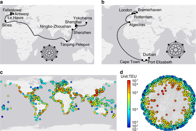
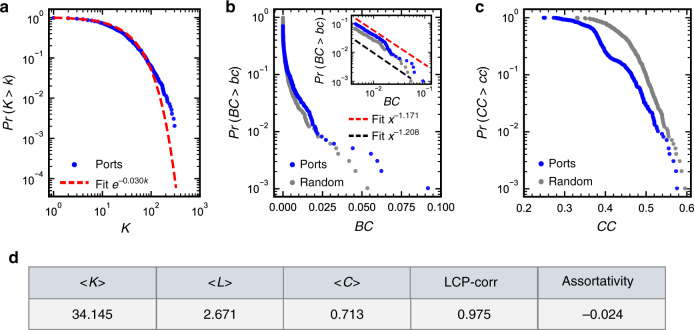
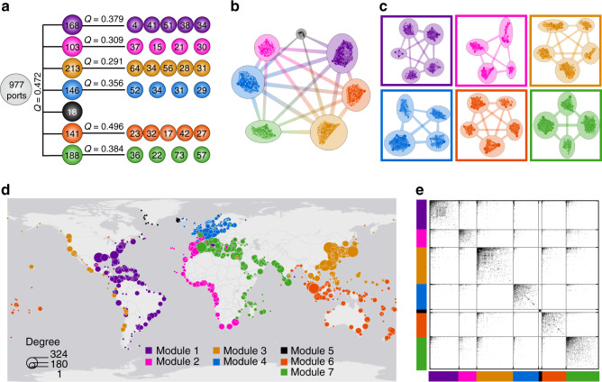
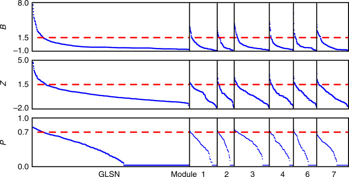
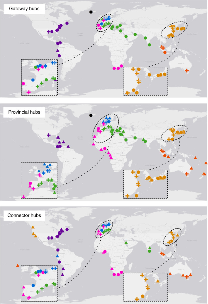
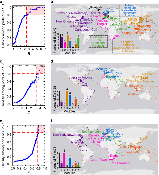
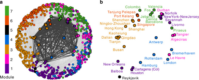
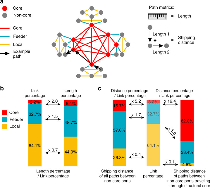
Around 80% of global trade by volume is transported by sea, and thus the maritime transportation system is fundamental to the world economy. To better exploit new international shipping routes, we need to understand the current ones and their complex systems association with international trade. We investigate the structure of the global liner shipping network (GLSN), finding it is an economic small-world network with a trade-off between high transportation efficiency and low wiring cost. To enhance understanding of this trade-off, we examine the modular segregation of the GLSN; we study provincial-, connector-hub ports and propose the definition of gateway-hub ports, using three respective structural measures. The gateway-hub structural-core organization seems a salient property of the GLSN, which proves importantly associated to network integration and function in realizing the cargo transportation of international trade. This finding offers new insights into the GLSN's structural organization complexity and its relevance to international trade.

Fig. 1. Construction of the global liner shipping network.

With the information on ports of call of world’s individual liner shipping service routes, we made each service route a complete graph where any two ports in the service route were connected via an edge. By merging the complete graphs derived from all individual liner shipping service routes, we obtained the GLSN. See “Methods”, for details about the adopted data on world’s liner shipping service routes and details about the adopted network topology representation method for GLSN construction. In (a and b), we show how complete graphs are derived from individual liner shipping service routes, with two examples: an Asia-Europe service route consisting of nine ports (a) and an Africa-Europe service route consisting of seven ports (b). In (c and d), we show ports of the GLSN using a geographical map and show inter-port connections using a hyperbolic layout obtained by coalescent embedding, respectively. The color of nodes corresponds to the traffic capacity of ports measured in Twenty-Foot Equivalent Unit (TEU). The coalescent embedding layout clearly points out that TEU gradient is related with the radial coordinate of the hyperbolic model, therefore ports with larger TEU values are more central in the hyperbolic geometry underlying the GLSN. The coalescent embedding hyperbolic layout locates at centre the nodes that are fundamental for the efficient navigability of a complex network. As such, the observed phenomenon that ports with larger TEU are more central in the hyperbolic layout means that ports with larger TEU are fundamental for the efficient navigability of the GLSN in transporting cargoes traded worldwide. This suggests that ports’ traffic capacity measured in TEU is indeed a meaningful indicator to be associated with international trade (as we will show in the rest of the study). Source data are provided as a Source Data file.

Fig. 2. Basic topological properties of the GLSN.

In (a), complementary cumulative distribution function of degree is reported in log-log scale (dots), fitted by an exponential function (dash line) instead of power-law; tests on the power-law distribution of the data failed based on the method of Clauset et al. and the method of Voitalov et al as well. Complementary cumulative probability distributions of betweenness centrality (BC) and closeness centrality (CC) for ports are plotted in semi-log scale in (b and c), respectively, in comparison to an equivalent random network which exactly keeps the same degree distribution as the original GLSN. The inset in (b) reports in log-log scale a power-law tail (red dash line) in the betweenness distribution with an exponent 1.171, corresponding to ports with BC ≥ 0.0043 (dots); power-law-ness is tested based on the method of Clauset et al.. For an equivalent random network, the betweenness distribution for nodes with BC ≥ 0.0043 decays with an exponent 1.208 (mean across 80.4% (804 out of 1000) iterations passing the test) (black dash line). The average closeness centrality of the GLSN (i.e., 0.382) is close to that of an equivalent random graph (i.e., 0.440, mean across 1000 iterations). The bottom panel d presents the average port degree <K>, average shortest path length <L>, average clustering coefficient <C>, degree assortativity coefficient and local-community-paradigm correlation (LCP-corr). To confirm these basic topological properties of the GLSN, we repeated the analysis by using the liner shipping service routes data of 2017. The results for the GLSN of 2017 are consistent with the present results for the GLSN of 2015 (Supplementary Fig. 1). Source data are provided as a Source Data file.

Fig. 3. Multiscale modular communities in the GLSN.

In (a–c), we give results for the division of both modular and submodular port communities. a Values of the modularity index (Q), together with the size of each module (i.e., number of ports); see “Methods” for a formal definition of Q. The network plots show the extracted modules (b) and the submodules (c); larger separation between models (submodules) is adopted to visualize the weaker connections between them, and inter-module (inter-submodule) connections are simplified. In (d and e), we show the results for the division of modular port communities. d A geographical plot presenting the seven modular communities by color. e A matrix plot presenting intra-module and inter-module links, with color black indicating a pair of ports are linked and color white unlinked; in each module ports are sorted in a descending order of degree.

Fig. 4. Ports’ outside-module degree (B), inside-module degree (Z), and participation coefficient (P).

The rank-size distributions of B, Z, and P of ports are presented in linear plots. The large plots on the left correspond to the results for modular communities in the GLSN, and the small plots on the right the results for submodular communities in individual modules (except for module 5, the smallest one that cannot be further divided into submodules); plots are scaled according to the corresponding number of ports. Dash lines in the plots indicate corresponding threshold values of 1.5, 1.5, and 0.7 used to define gateway hubs, provincial hubs, and connector hubs, respectively.

Fig. 5. Geographical distribution of hub ports in the GLSN.

Here the three plots show the gateway-hub ports (i.e., ports with B ≥ 1.5), provincial-hub ports (i.e., ports with Z ≥ 1.5), and connector-hub ports (i.e., ports with P ≥ 0.7), respectively. Ports are colored according to modular communities. In each plot, triangles denote ports which have only that particular type of hub role under investigation; circles, ports which have one additional type of hub role; crosses, ports which have all the three types of hub roles. Outside-module degrees (B), inside-module degrees (Z), and participation coefficients (P) of the hub ports are reported in the source data. Source data are provided as a Source Data file.

Fig. 6. Structural core detection of the GLSN.

A structural core of the GLSN is defined as a set of hub ports that meet two criteria: first, this set should consist of the largest number of the most important hub ports that form a subgraph of high density (i.e., here at least 0.8); second, this set should contain at least one hub port from each module in the network. In implementation, we first calculated the connection densities among ports with largest values of B, Z, and P, as presented in plots a, c, and e, respectively. Red regions in the parameter spaces of these three plots correspond to the three respective sets of hub ports that meet the first criterion: ports of B ≥ 2.43, forming a subgraph of density 0.80; ports of Z ≥ 3.25, forming a subgraph of density 0.82; and ports of P ≥ 0.78, forming a subgraph of density 0.85. These three sets of hub ports are further displayed by big dots in geographical plots b, d and f, as well as their respective distributions over different modules (insets). Then, we could evaluate whether any of the three sets meet the second criterion. It turned out that only the set of ports of B ≥ 2.43 met this criterion and thus constituted a structural core of the GLSN, while the other two sets did not. Modules are indicated by color. Pseudocode of the algorithm for structural core detection is available in Supplementary Note 7.

Fig. 7. Representation of the GLSN and its structural core in the hyperbolic space.

The color of the nodes corresponds to the modular communities. In (a), the nodes belonging to the structural core are highlighted with a thicker black border and the intra-core connections are marked in dark gray, whereas the other connections are in light gray. Names of the structural-core ports are indicated in (b). The detected gateway-hub structural-core is at the center of the hyperbolic layout. Nodes at the center of this layout are crucial to support the efficient navigability of a complex network. From a previous analysis we know that these nodes at the center have also larger TEU (as presented in Fig. 1d). This indicates that the gateway-hub structural core is indeed mainly composed by ports with larger TEU that are fundamental for efficient navigability of the network in transporting cargoes traded worldwide. Therefore, structural-core ports are important candidates to be associated with international trade (as we will analyse in the next section). In order to be sure that the hyperbolic representation is meaningful and the community separation is significantly and properly represented in the hyperbolic layout, we computed an index of angular separation of the communities (ASI) in respect to the worst scenario in which the nodes of each community are equidistantly distributed over the circumference. This index is in the range [0,1]: 0 indicates the worst case, and 1 indicates a case of perfect angular separation. For the provided embedding the ASI is 0.7, which represents a good angular separation of the communities in the embedding space and is statistically significant with a p-value < 0.001 (see Supplementary Fig. 4 for details on the statistical test).

Fig. 8. Statistics of the core, feeder and local connections.

a Schematic illustration of path metrics; the geographical length of an inter-port connection is measured as the real nautical distance (https://www.searates.com/services/distances-time/) between the two ports, and shipping distance of any port pair is the sum of geographical length of edges along the shortest path. b Ratios of length percentage to link percentage for core connections, feeder connections and local connections, respectively. c Percentages of core connections, feeder connections and local connections in the total shipping distance of all shortest paths between non-core ports (left bar), and of shortest paths between non-core ports which travel through the structural core (right bar). To better understand those three types of connections related with the structural-core organization of the GLSN, one is encouraged to refer to the hub-and-spoke service network configuration (Hu and Zhu), which is widely adopted by world liner shipping carriers in practice. The hub-and-spoke configuration is illustrated in the Supplementary Fig. 5. In addition, we estimated the physical length of an inter-port connection as the great-circle distance based on ports’ geographical locations of latitude and longitude, and then repeated the analysis. We found all the results reported here remain almost invariant (Supplementary Note 8).

Fig. 9. Correlation between the GLSN topological indicators and international trade indicators of countries.

In (a), we show for countries the Pearson correlation coefficients between international trade value (ITV) and # all (inter-port) connections with all other countries in the world (black bar); between ITV and # SC connections (structural-core connections, those between a country’s structural-core ports and ports of other countries), yellow bar; and between ITV and # NSC connections (non-structural-core connections, those between a country’s non-structural-core ports and ports of other countries), green bar. In (b), we show for country pairs the Pearson correlation coefficients between the bilateral trade value (BTV) and # all (inter-port) connections between the two countries (black bar); between BTV and # SC connections (structural-core connections, those with at least one end-node of the connection being a structural-core port), yellow bar; and between BTV and # NSC connections (non-structural-core connections, those with two end-nodes of the connection being both non-structural-core ports), green bar. We test the statistical significance of the results reported for SC connections (yellow bars), by randomly selecting 1000 sets of ports corresponding in size to the number of ports contained in the structural core (which is 37) and repeating for each random set of ports the same analysis as we did for the detected structural core. Gray bars show the averages of 1000 random cases, and error bars report the standard errors. Source data are provided as a Source Data file.

References

1. UNCTAD. Review of Maritime Transport 2017. https://unctad.org/en/pages/publicationwebflyer.aspx?publicationid=1890 (2017).
1. Bernhofen DM, El-Sahli Z, Kneller R. Estimating the effects of the container revolution on world trade. J. Int. Econ. 2016;98:36–50.
1. Limão N, Venables AJ. Infrastructure, geographical disadvantage, transport costs, and trade. World Bank Econ. Rev. 2001;15:451–479.
1. Clark X, Dollar D, Micco A. Port efficiency, maritime transport costs, and bilateral trade. J. Dev. Econ. 2004;75:417–450.
1. Bar-Yam Y. Dynamics of Complex Systems. Cambridge, MA: Westview Press; 1997.
Publication types