Characterizing physiological and symptomatic variation in menstrual cycles using self-tracked mobile-health data

Abstract

The menstrual cycle is a key indicator of overall health for women of reproductive age. Previously, menstruation was primarily studied through survey results; however, as menstrual tracking mobile apps become more widely adopted, they provide an increasingly large, content-rich source of menstrual health experiences and behaviors over time. By exploring a database of user-tracked observations from the Clue app by BioWink GmbH of over 378,000 users and 4.9 million natural cycles, we show that self-reported menstrual tracker data can reveal statistically significant relationships between per-person cycle length variability and self-reported qualitative symptoms. A concern for self-tracked data is that they reflect not only physiological behaviors, but also the engagement dynamics of app users. To mitigate such potential artifacts, we develop a procedure to exclude cycles lacking user engagement, thereby allowing us to better distinguish true menstrual patterns from tracking anomalies. We uncover that women located at different ends of the menstrual variability spectrum, based on the consistency of their cycle length statistics, exhibit statistically significant differences in their cycle characteristics and symptom tracking patterns. We also find that cycle and period length statistics are stationary over the app usage timeline across the variability spectrum. The symptoms that we identify as showing statistically significant association with timing data can be useful to clinicians and users for predicting cycle variability from symptoms, or as potential health indicators for conditions like endometriosis. Our findings showcase the potential of longitudinal, high-resolution self-tracked data to improve understanding of menstruation and women's health as a whole.

Keywords: Data mining; Data processing.

Fig. 1. Clue app screenshot.

Sample screenshots of the Clue app. Users can track daily symptoms across 20 categories; Table 3 provides a description of the available Clue categories and their corresponding symptoms. On the left for example, the app displays what day the user is currently on in their cycle. On the right, a user can choose from ‘cramps,’ ‘headache,’ ‘ovulation,’ or ‘tender breasts’ symptoms for the category ‘pain’ (the third most tracked category in our dataset, see Table 3). Screenshots produced by and used with permission from Clue by BioWink GmbH.

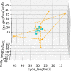
Fig. 2. Time series embedding for cycle length (one user, across groups).

We sample one consistently highly variable and one consistently not highly variable user, each with the median number of cycles (11), from the user cohort and plot each set of three consecutive cycles on the x, y, and z axes, respectively. This allows us to visualize how much a user’s cycle lengths change throughout their entire cycle tracking history—we would expect that a not consistently highly variable user would have points that cluster closer together in space. We see that the consistently not highly variable (teal) user occupies a small region, while the consistently highly variable (orange) user’s points move through the space. This indicates that the teal user’s cycle lengths are consistently very similar to one another, whereas the orange user experiences more consistent fluctuation in cycle lengths. Thus, we see that separating users into groups on the basis of median CLD identifies those who are more and less consistently highly variable.

Fig. 3. Time series embedding and probability distribution for cycle length (all users, across groups).

Time series embedding (a) and probability distributions (b) of cycle length for the consistently not highly variable (teal) and consistently highly variable (orange) groups. a The cycle lengths of three consecutive randomly sampled cycles from each user in the cohort are plotted on the x, y, and z axes. Each consistently not highly variable user is represented by a teal point, and each consistently highly variable user by an orange point. It is visually evident that the teal cluster of users occupies a tighter region of the space around the x = y = z line, with the orange cluster fanning outward. b The cycle length probability distributions of the cohort, where we note that the orange group’s distribution has a much wider spread and is less peaked than the teal group. Cycle lengths are more heterogeneous or widely distributed for the orange group, confirming that the consistently highly variable group represents those with more fluctuation in cycle length. The cumulative distributions per group differ significantly (as per a two-sample Kolmogorov–Smirnov test).

Fig. 4. Time series embedding and probability distribution for period length (all users, across groups).

Time series embedding (a) and probability distributions (b) of period length for the consistently not highly variable (teal) and consistently highly variable (orange) groups. a The period lengths of three consecutive randomly sampled cycles from each user in the cohort are plotted on the x, y, and z axes. Visually, we observe that both groups occupy a very similar region of the period length space (few orange points are placed outside the region occupied by the teal cluster). b The period length probability distributions of the cohort, where we observe that the orange and teal distributions are largely overlapping, with the same median of 4 days and a similar shape, indicating that period lengths are distributed very similarly for the two groups. We notice a slight peak in single day period reports in both groups, which we argue is reminiscent of app usage behavior: some users are interested in knowing (approximately) when they had their period, not in tracking how long it was, so they may only track the day it occurred and not continue tracking after that.

Fig. 5. Average cycle and period length by cycle ID.

For each user’s cycles (indexed by cycle ID), we average cycle (a) and period length (b) across three different groups: the entire user cohort (top, purple), the consistently not highly variable user cohort (middle, teal), and the consistently highly variable user cohort (bottom, orange). This allows us to visualize how cycle and period length vary over time for each group on average and in terms of standard deviation (for illustrative purposes, we restrict the cycle ID to 20). Cycle and period length statistics are stationary over the app usage timeline within each plot. We note that the top and middle plots look similar in each figure (i.e., the consistently not highly variable group looks similar to the overall population in terms of both cycle and period length), but the wider shaded orange spread of the bottom plot demonstrates the higher degree of variability in the consistently highly variable group. In addition, this spread is consistently wider for the orange plot over time. This showcases that the consistently highly variable group represents a large degree of the variability that we see in the data overall.

Fig. 6. Filtering process for computing user and cycle cohort.

Step-by-step filtering process for computing the final user and cycle cohort. The percentage of users and cycles removed at each step is computed out of the initial numbers. Note that we only include users aged between 21 and 33 years, since women exhibit more stable menstrual behavior in their ‘middle life’ phase^,,,,.

Fig. 7. Identifying cycle tracking artifacts and characterizing user regularity.

We provide illustrative examples of identifying a cycle tracking artifact (top) and characterizing a user’s regularity (bottom) based on CLD statistics. In each example, we display a user’s cycle history with a total of four cycles. Cycle length is computed as the length of time between the first day of a period and the first day of the next period, and CLD is computed as the absolute difference between subsequent cycle lengths (i.e., if a user has n cycles tracked, they will have n − 1 CLD values). Period length is computed by counting the number of sequential days on which there is menstrual bleeding greater than spotting (‘light,’ ‘medium,’ or ‘heavy’). Two such sequences are considered one period if separated by no more than one day of non-bleeding/spotting. In the top example, the user’s second CLD exceeds their median by at least 10, and thus we identify the corresponding ‘artifically long’ cycle in red—this cycle will be excluded from our analysis. In the bottom example, the user’s median CLD is at least 9, and thus they will be classified as a consistently highly variable user.

Fig. 8. Histogram of maximum CLD before and after excluding cycle artifacts.

For each user, we compute the maximum CLD and plot a histogram before (blue) and after (red) excluding cycles without user engagement (i.e., cycles that are potential artifacts). We see that the multimodal behavior (peaks at around 30 and 60 days) is largely dampened upon removing these cycles. In addition, the fat right-hand tail in the red curve implies that we preserve the natural variation in cycle length—we are not simply removing long cycles.

Fig. 9. Median CLD versus maximum CLD two-dimensional histogram.

We plot a two-dimensional histogram of users’ median CLD versus maximum CLD in logarithmic space, as well as the line where maximum CLD is equal to median CLD plus 10 in red. We can see that the line separates out a highly concentrated region of users, as well as a more scattered region of users. Specifically, the majority of the mass falls under this line, as showcased by the concentrated red color in the lower left-hand corner of the plot, and a diagonal band extending upward, while the region above the line is more spread out. Thus, we examine the cycles that fall above the line as possible cycle tracking artifacts.

Fig. 10. Cumulative distribution of median CLD.

Looking at the cumulative distribution of median CLD, we see that the curve flattens out significantly around the ‘elbow’ at 9 days; thus, we choose greater than 9 days as our cutoff for our definition of consistently highly variable.

References

1. Popat VB, Prodanov T, Calis KA, Nelson LM. The menstrual cycle: a biological marker of general health in adolescents. Ann. N. Y. Acad. Sci. 2008;1135:43–51. - PMC - PubMed
1. Bedford JL, Prior JC, Barr SI. A prospective exploration of cognitive dietary restraint, subclinical ovulatory disturbances, cortisol, and change in bone density over two years in healthy young women. J. Clin. Endocrinol. Metab. 2010;95:3291–3299. - PubMed
1. Zittermann A, et al. Physiologic fluctuations of serum estradiol levels influence biochemical markers of bone resorption in young women. J. Clin. Endocrinol. Metab. 2000;85:95–101. - PubMed
1. Solomon CG, et al. Menstrual cycle irregularity and risk for future cardiovascular disease. J. Clin. Endocrinol. Metab. 2002;87:2013–2017. - PubMed
1. Carmina E, Lobo RA. Polycystic ovary syndrome (PCOS): arguably the most common endocrinopathy is associated with significant morbidity in women. J. Clin. Endocrinol. Metab. 1999;84:1897–1899. - PubMed