Properties of structural variants and short tandem repeats associated with gene expression and complex traits

Abstract

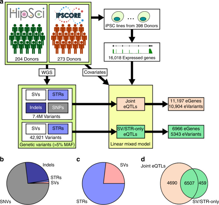
Structural variants (SVs) and short tandem repeats (STRs) comprise a broad group of diverse DNA variants which vastly differ in their sizes and distributions across the genome. Here, we identify genomic features of SV classes and STRs that are associated with gene expression and complex traits, including their locations relative to eGenes, likelihood of being associated with multiple eGenes, associated eGene types (e.g., coding, noncoding, level of evolutionary constraint), effect sizes, linkage disequilibrium with tagging single nucleotide variants used in GWAS, and likelihood of being associated with GWAS traits. We identify a set of high-impact SVs/STRs associated with the expression of three or more eGenes via chromatin loops and show that they are highly enriched for being associated with GWAS traits. Our study provides insights into the genomic properties of structural variant classes and short tandem repeats that are associated with gene expression and human traits.

Fig. 1. eQTL mapping.

a Overview of eQTL study design. We performed two eQTL analyses: a joint analysis that used all variants and identified 11,197 eGenes and an SV/STR-only analysis that only used SVs and STRs and identified 6,996 eGenes. b,c Pie charts showing the number of lead variants across the different variant classes for (b) joint and (c) SV/STR-only eQTL analyses. d Venn diagram showing the intersection between the eGenes detected in the joint and the SV/STR-only analysis.

Fig. 2. Variant length influences the likelihood and effect size of eQTLs.

a Percentage of variants with length greater than the thresholds on the x axis that were eVariants (grey lines) or lead eVariants (green lines). Points are colored according to the enrichment (log 2 odds ratio) of variants above each threshold among eVariants or lead eVariants relative to variants smaller than the threshold; points circled in red were significant (FET two-sided, p < 0.05). A complete list of p values and odds ratios is provided in Supplementary Fig. 4. (b,c) Association of variant length with eQTL effect size for (b) non-exonic eQTLs or (c) exonic eQTLs mapped to biallelic deletions (n = 1,769 non-exonic, n = 48 exonic), duplications (n = 235 non-exonic, n = 13 exonic), multi-allelic CNVs (n = 1,278 non-exonic, n = 111 exonic) and STRs (n = 13,085 non-exonic, n = 148 exonic). Number of eQTLs for each variant class at defined length is shown in top panels. Points in bottom panels represent the centers of bins with equal numbers of observations and error bars indicate 95% confidence intervals around the mean (1000 bootstraps). Lines represent linear regressions, with 95% confidence intervals shaded, as calculated on unbinned data. p values at the right of each plot indicate the significance of the association between length and absolute effect size (linear regression, t-test) in a model that includes non-mode allele frequency and distance to TSS as covariates. p values presented are not adjusted for multiple testing.

Fig. 3. Properties of SV and STR eQTLs.

a Percentage of tested variants from each class that are eVariants (eV), left) or lead eVariants (right) in the SV/STR-only eQTL. Asterisks indicate significant enrichment or depletion of variants among eVariants relative to STRs (FET two-sided, BH alpha < 0.05). b Left panel is a balloon plot where color indicates number of eVariants and size indicates fraction of eVariants in each bin. Right panel shows average number of eGenes per eVariant with 95% confidence intervals. Red points indicate significantly higher numbers of eGenes per eVariant (Mann–Whitney U one-sided, Bonferonni p < 0.05) compared to STRs. c Distribution of the distance of eQTL (left) and lead eQTL (right) variants to the boundary of their eGenes. Percentages indicate the proportion of eQTLs that were at least 250 kb distal to eGene, red asterisks indicate that eQTLs tended to be localized farther from eGenes as compared to STRs (Mann–Whitney U Test one-sided, Bonferonni p < 0.05). Distributions for lead SNV and indel eQTLs were not examined for significant differences relative to STRs. d Fraction of lead eQTLs that were intergenic or overlapped exons, promoters, or introns of their associated eGene or other genes. e Enrichment of lead eQTLs for each class that overlap each genic element compared to variants from all other classes (FET two-sided, BH alpha < 0.05). f Distribution of effect sizes for lead eQTLs that overlapped or did not overlap an exon of their eGene. (G,H) Distribution of absolute effect sizes for SV classes, STRs, and SNV/indels for exonic (g) and non-exonic (h) eQTLs. Vertical dashed lines indicate means. P values are derived from comparing the effect size distributions for mCNVs to the distributions for STRs, SVs, SNVs, and indels (Mann–Whitney U test one-sided, Bonferonni p < 0.05). All p values and odds ratios for (a) and (e) are in Supplementary Figs. S5 and S6. eQTL statistics for SNV and indels are from the joint analysis for all panels.

Fig. 4. Properties of eGenes associated with different variant classes.

a Fraction of eGenes of each Gencode gene subtype mapped to lead variants of each class for the SV/STR-only eQTL. b Enrichment of the proportion of eGenes of each subtype mapped to a variant class compared with the proportion of other eGenes falling into that subtype. Significant associations (FET, BH FDR < 0.05) are indicated with x symbols. c Absolute effect size of associations for genes of each subtype among lead eQTLs. P values indicate significance of Mann–Whitney U test (one-sided) for difference in the effect size distributions of each category compared to protein coding genes (Bonferroni). For boxplots the minimum box edge indicates the first quartile while the maximum box edge indicates the third quartile and the center line indicates the median value. Whiskers of the box plot are drawn at the maximum point (upper whisker) or minimum point (lower whisker) that is within 1.5 times the interquartile range (quartile three—quartile one). d Distribution of ExAC scores for intolerance to loss-of-function variants in a single allele (pLI, red), intolerance to loss-of-function variants in both alleles (pRec, orange), and tolerance to loss-of-function variants in both alleles (pNull, blue) for 5,675 eGenes. e The percentage of eGenes (grey bars) mapped to lead variants that had high (>0.9) pLI (left), pRec (center), or pNull scores (right). Black bars show percentages for 7,337 non-eGenes from the SV/STR-only analysis. P values indicate the significance of the difference between the proportion of high score eGenes and high score non-eGenes for each group individually (FET, BH FDR < 0.05, within each probability score). f Absolute effect size versus pLI score for all eGenes with a pLI score (n = 5,675). Points are equally-sized bins and error bars show 95% confidence intervals (n = 1000 bootstraps) around the mean pLI. Line is a model predicting pLI by eQTL effect size after regressing out variant class and mean log₁₀(TPM) expression level of the gene among expressed samples. p value is for the eQTL effect size term (t test).

Fig. 5. Localization of eQTLs near chromatin loops.

a Diagram showing localization of SVs and STRs at loop anchors. eVariants closer to the distal anchor (right of grey dotted line) than the promoter anchor were considered loop-acting eQTLs. b Proportion of eQTLs that were genic (yellow), overlapping or close to distal anchors (green), or distal acting by some other mechanism (grey). c Distal loop-acting eQTLs (n = 2,327 eQTLs for 1,598 eGenes) per SV class. d Percentage of eVariant-eGene pairs where the eVariant (left) or lead eVariant (right) overlaps or does not overlap the distal anchor. p values derived by comparing proportions for each class (FET two sided, Benjamini–Hochberg). e Fraction of tested distal variant-gene pairs (a) that were lead eQTLs versus their distance to the distal anchor. Points represent the means of equally-sized bins; errors bars 95% confidence intervals. Curves are logistic regressions using distance to the loop anchor to predict whether the variant-gene pair was a lead association. Regressions were computed separately for variant-gene pairs inside the loop (left, n = 47,831) or outside the loop (right, n = 294,796). Center panel shows fraction of variant-gene pairs that overlapped distal anchors and were lead eQTLs (n = 41,794). f Number of eVariants connected to gene promoters through chromatin loops (x-axis) and number of these connected genes that are eGenes (y-axis). g,h Percentage of tested variants that were eVariants (g) or lead eVariants (h) stratified by number of genes the variant was linked to through a distal anchor. p values for each bar were derived by comparing the proportion of tested variants that were eVariants and linked to genes to the proportion of variants that were eVariants and not linked to genes (first bar). i Number of eGenes versus number of tested genes per eVariant stratified by whether the genes are linked by loops to the eVariant (blue) or not linked by loops (grey). Lines indicate relationship between number of eGenes per eVariant and number of genes tested for genes that were or were not linked by loops. p value is for loop/nonloop term (t-test).

Fig. 6. Associations between SVs, STRs and GWAS.

a Distribution of maximum LD score per i2QTL variant with UKBB variants within 50 kb for each variant type. p values calculated for the LD distribution of each SV class relative to STRs (Mann––Whitney U, Bonferroni). b Fraction of variants of each class that are tagged by a UKBB variant (R² > 0.8) for lead eVariants (green) versus all other variants in that class (black). Q values indicate enrichment of lead eVariants to be in LD with a UKBB variant versus all other variants tested in the eQTL in the class (FET two-sided, Benjamini–Hochberg). c Fraction of variants of each class that are tagged by a UKBB variant that is associated with at least one trait in the UKBB (p < 5e-8). q values indicate enrichment of lead eVariants to be in strong LD with a UKBB variant that is associated with at least one trait versus all other variants tested in the eQTL in the class (FET two-sided, Benjamini–Hochberg). d Percentage of variants in LD (R² > 0.8) with a variant significantly linked to at least one GWAS trait when significantly associated with 0, 1, or 2 eGenes or more. To compute annotated q values, we utilized all variants tested in the SV/STR-only eQTL, and for each variant class we performed logistic regression to determine whether the number of eGenes for a variant was associated with whether the variant was in strong LD with a significant GWAS variant (z-test, Benjamini–Hochberg). e Example multi-gene eSTR on chromosome 22 with nine unique eGenes (pink/red) including four genes that the STR loops to. Genes for which the variant is a lead variant are colored red. iPSC Hi-C data is visualized as a heatmap of interaction frequencies. The variant is located between two chromatin subdomains that span ~100 kb on the left side of the variant and ~25 kb on the right side of the variant. f Example of an mCNV on chromosome 7 that is a multi-gene eQTL associated with seven unique eGenes by looping. Exact p values and odds ratios for (b) and (c) are in Supplemental Fig. 12.

References

1. Chiang C, et al. The impact of structural variation on human gene expression. Nat. Genet. 2017;49:692–699. - PMC - PubMed
1. Schlattl A, Anders S, Waszak SM, Huber W, Korbel JO. Relating CNVs to transcriptome data at fine resolution: Assessment of the effect of variant size, type, and overlap with functional regions. Genome Res. 2011;21:2004–2013. - PMC - PubMed
1. Sudmant PH, et al. An integrated map of structural variation in 2,504 human genomes. Nature. 2015;526:75–81. - PMC - PubMed
1. Jakubosky, D. et al. Discovery and quality analysis of a comprehensive set of structural variants and short tandem repeats. Nat Commun. 10.1038/s41467-020-16481-5 (2020). - PMC - PubMed
1. Li X, et al. The impact of rare variation on gene expression across tissues. Nature. 2017;550:239–243. - PMC - PubMed
Publication types