Discovery and quality analysis of a comprehensive set of structural variants and short tandem repeats

Abstract

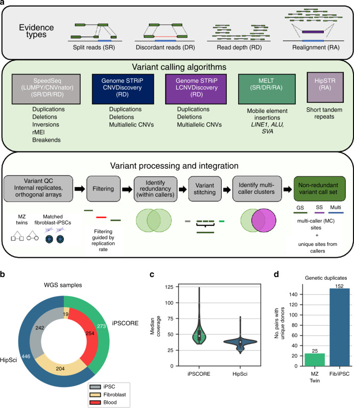
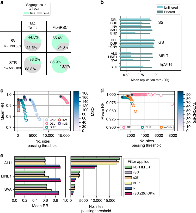
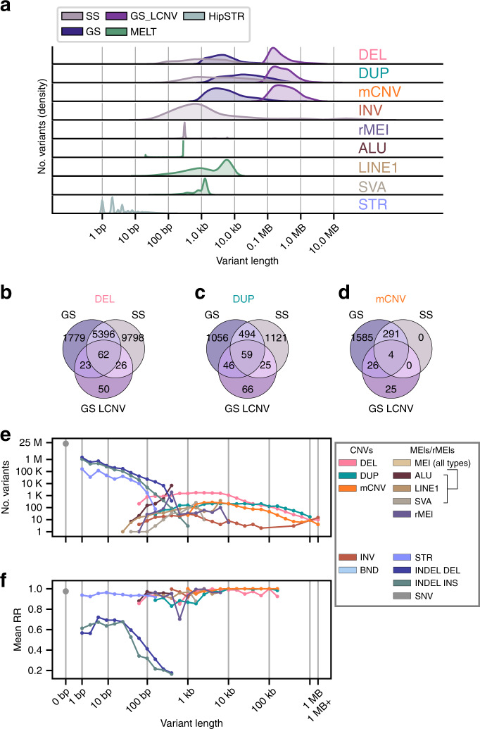
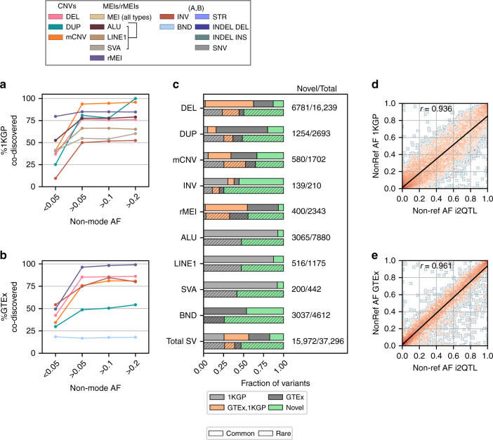
Structural variants (SVs) and short tandem repeats (STRs) are important sources of genetic diversity but are not routinely analyzed in genetic studies because they are difficult to accurately identify and genotype. Because SVs and STRs range in size and type, it is necessary to apply multiple algorithms that incorporate different types of evidence from sequencing data and employ complex filtering strategies to discover a comprehensive set of high-quality and reproducible variants. Here we assemble a set of 719 deep whole genome sequencing (WGS) samples (mean 42×) from 477 distinct individuals which we use to discover and genotype a wide spectrum of SV and STR variants using five algorithms. We use 177 unique pairs of genetic replicates to identify factors that affect variant call reproducibility and develop a systematic filtering strategy to create of one of the most complete and well characterized maps of SVs and STRs to date.

Fig. 1. Variant calling, processing, and i2QTL WGS samples.

a Illustration of the evidence types from short read sequencing data utilized in variant calling (top). Description of the variant callers utilized, the types of variants they identify, and the evidence they use (middle). Flowchart showing the processing, quality control (see Methods), and integration of SVs from different variant callers (bottom). b Pie chart showing the number of whole-genome sequencing samples from the iPSCORE or HipSci studies used for variant calling and the cell type from which DNA was obtained. c Distribution of the median coverage of whole genomes from iPSCORE (n = 273) (green) and HipSci (n = 446) (blue). Boxplots are contained within violinplots, and the minimum box edge indicates the first quartile while the maximum box edge indicates the third quartile. White dots in the boxes indicate the median value. Whiskers of the box plot are drawn at the maximum point (upper whisker) or minimum point (lower whisker) that is within 1.5 times the interquartile range (quartile three–quartile one). Points beyond this range are considered outliers (and not plotted) but maximum and minimum values are shown with the range of the outer violinplot. d Number of genetic replicate samples included in the collection, including 25 monozygotic twin pairs (iPSCORE) and fibroblast–iPSC pairs from 152 unique donors (HipSci). These data enable robust variant calling for all classes of genetic variation along with reproducibility analysis.

Fig. 2. Replication rate is associated with reported quality metrics.

a Proportion of SVs and STRs that were non-reference (green) in at least one of the iPSCORE MZ twin pairs or HipSci fibroblast–iPSC pairs prior to filtering. b Replication rate of variants before and after filtering and deduplicating within caller; Genome STRiP and SpeedSeq abbreviated in figure as GS and SS respectively. c Replication rate in MZ twins versus the number of total SpeedSeq (LUMPY) sites remaining that pass criteria when filtering variants to different thresholds for MSQ score (indicated by color). d Replication rate versus the number of total Genome STRiP sites remaining that pass criteria when filtering variants to different thresholds for GSCNQUAL score (indicated by color). e Replication rate in MZ twins for MELT sites that pass criteria when filtering variants under suggested hard site filters (left). Pink represents the result of filtering using all four exclusion criteria (rSD, s25, hDP, lc; see Methods). The number of total sites remaining that passed criteria is shown at right.

Fig. 3. Variant length distributions and variant caller comparison.

a Density plot showing the size spectrum of each variant caller before identifying multi-caller clusters. b–d Number of overlapping variants after identifying multi-caller clusters for deletions (b), duplications (c), and mCNVs (d). e Number of variants in the non-redundant call set separated by variant class and grouped in log linear bins by variant length. Points are drawn at the upper limit of each bin (e.g. a bin from 50 to 100 bp is drawn at 100 bp). For STRs length represents the maximum number of bases different from the reference at each site (largest insertion or deletion observed). f The average replication rate of variants segregating in the 25 monozygotic twin pairs is represented for each length bin that contains at least 10 variants. GATK SNVs and indels previously discovered in iPSCORE samples were used for e and f.

Fig. 4. Comparison to other SV calling studies.

a, b The fraction of variants from either a 1KGP (European population) or b GTEx that were also captured in our study in different non-mode allele frequency (NMAF) bins. c Fraction of i2QTL SVs that were co-discovered in 1KGP, GTEx, both 1KGP and GTEx, or were unique to i2QTL (novel), divided by whether variants were common (>0.05 NMAF) or rare (<0.05 NMAF) in unrelated i2QTL samples indicated by absence or presence of hatching respectively. d, e Non-reference allele frequency of variants co-discovered in i2QTL and d 1KGP (Europeans) or e GTEx in their respective discovery samples. Here, the non-reference allele frequency among unrelated i2QTL donors is used, and the density is plotted with orange indicating more observations, and blue fewer.

Fig. 5. Linkage disequilibrium tagging of structural variants and short tandem repeats.

Distribution of maximum linkage disequilibrium (R²) in i2QTL Europeans between common SVs and STRs (non-mode allele frequency > 0.05) and SNVs or indels within 50 kb, considering only SVs/STRs that are within 1 MB of an expressed gene in iPSCs.

References

1. Carvalho CM, Lupski JR. Mechanisms underlying structural variant formation in genomic disorders. Nat. Rev. Genet. 2016;17:224–238. - PMC - PubMed
1. Brandler WM, et al. Paternally inherited cis-regulatory structural variants are associated with autism. Science. 2018;360:327–331. - PMC - PubMed
1. Malhotra D, et al. High frequencies of de novo CNVs in bipolar disorder and schizophrenia. Neuron. 2011;72:951–963. - PMC - PubMed
1. Malhotra D, Sebat J. CNVs: harbingers of a rare variant revolution in psychiatric genetics. Cell. 2012;148:1223–1241. - PMC - PubMed
1. Michaelson Jacob J, et al. Whole-genome sequencing in autism identifies hot spots for de novo germline mutation. Cell. 2012;151:1431–1442. - PMC - PubMed
Publication types