Phylogenetic background and habitat drive the genetic diversification of Escherichia coli

Abstract

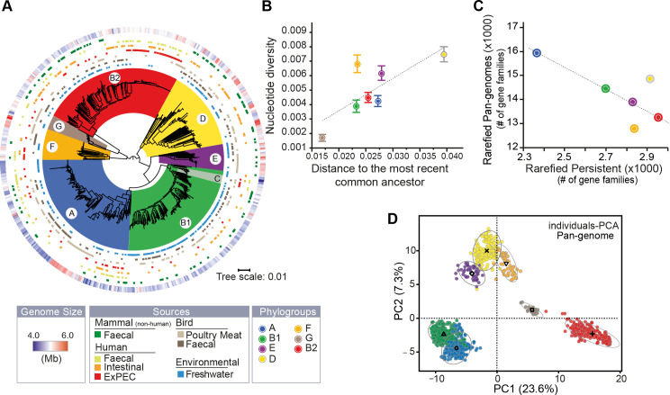
Escherichia coli is mostly a commensal of birds and mammals, including humans, where it can act as an opportunistic pathogen. It is also found in water and sediments. We investigated the phylogeny, genetic diversification, and habitat-association of 1,294 isolates representative of the phylogenetic diversity of more than 5,000 isolates from the Australian continent. Since many previous studies focused on clinical isolates, we investigated mostly other isolates originating from humans, poultry, wild animals and water. These strains represent the species genetic diversity and reveal widespread associations between phylogroups and isolation sources. The analysis of strains from the same sequence types revealed very rapid change of gene repertoires in the very early stages of divergence, driven by the acquisition of many different types of mobile genetic elements. These elements also lead to rapid variations in genome size, even if few of their genes rise to high frequency in the species. Variations in genome size are associated with phylogroup and isolation sources, but the latter determine the number of MGEs, a marker of recent transfer, suggesting that gene flow reinforces the association of certain genetic backgrounds with specific habitats. After a while, the divergence of gene repertoires becomes linear with phylogenetic distance, presumably reflecting the continuous turnover of mobile element and the occasional acquisition of adaptive genes. Surprisingly, the phylogroups with smallest genomes have the highest rates of gene repertoire diversification and fewer but more diverse mobile genetic elements. This suggests that smaller genomes are associated with higher, not lower, turnover of genetic information. Many of these genomes are from freshwater isolates and have peculiar traits, including a specific capsule, suggesting adaptation to this environment. Altogether, these data contribute to explain why epidemiological clones tend to emerge from specific phylogenetic groups in the presence of pervasive horizontal gene transfer across the species.

Fig 1. The genetic diversity of Australian E. coli.

A. Distribution of isolates per region and per source. B. The pan-genome is composed of 75,890 gene families, of which 33,705 are singletons (in green, present in a single genome), 2,486 persistent (in gold, present in at least 99% of genomes), the remaining being accessory (in grey). 29,657 gene families (39% of the pan-genome) were related to mobile genetic elements (MGE). C. Functional EggNOG categories of pan-genome gene families. The ratio observed/expected (O/E) for the frequency of non-supervised orthologous groups (NOGs, shown as capitalized letters) is reported for all comparisons with a color code ranging from blue (under-representation) to red (over-representation). The level of significance of each Fisher’s exact test was indicated (P> = 0.05 : ns; P<0.05 : *; P<0.01 : **; P<0.001 :***). It was performed on each 2*2 contingency table. Gene families lacking matches to the EggNOG functional categories were discarded. D. Percentage of the different EggNOG categories (see insert) in the persistent, accessory and singleton gene families and among genes associated to MGE.

Fig 2. Evolution of Gene Repertoire Relatedness (GRR) with time.

A. [Top] Violin plots of the patristic distance computed between pairs of intra-ST (in blue), inter-ST (in purple), and inter-phylogroup (in water green) genomes. [Bottom] Association between GRR and the patristic distance across pairs of genomes. Due to the large number of comparisons (points), we divided the plot area in regular hexagons. Color intensity is proportional to the number of cases (count) in each hexagon. The linear fit (black solid line, linear model (lm)) was computed for the entire dataset (1,294 genomes, Y = 90.2–75.7*X, R² = 0.49, P<10⁻⁴). The spline fit (generalized additive model (gam)) was computed for the whole (in black dashed line) or the intra-ST (in blue solid line) comparisons. There was a significant negative correlation between GRR and the patristic distance (Spearman’s rho = -0.67, P<10⁻⁴). B. Stacked bar plot of the number of intra-ST (in blue) and inter-ST (in purple) comparisons at short evolutionary scales. C. Violin plots of the intra-ST, inter-ST and inter-phylogroup GRR (%). (A-B-C) All the distributions were significantly different (Wilcoxon test, P<10⁻⁴), the same color code was used and described in panel A.

Fig 3. The genetic and ecological structure of Australian E. coli population.

A. Phylogenetic tree of E. coli rooted using the genomes of other Escherichia (only shown in S4 Fig for clarity). From the inside to the outside: the 7 main phylogroups (arcs covering the tree), the source of each genome (seven rows), and the size of the genomes (outer row, see insert legend). B. Association between the nucleotide diversity per site (Pi, average and s.e) within phylogroup and their distance to their most recent common ancestor (MRCA). In each pylogroup, we averaged the nucleotide diversity (π) obtained for 112 core-genes, and the length branches (from tip-to-MRCA) of the species tree. C. Association between the rarefied pan- and persistent-genomes in each phylogroup. We used 1,000 permutations (genomes orderings) of 50 randomly selected genomes (rarefied datasets) to compute the pan- and the persistent-genomes in each phylogroup (ignoring the G group), and then averaged the results. D. Principal component analysis of the pan-genome (matrix of presence/absence of each gene family across genomes). Each dot corresponds to a genome in the two first principal components (PC). The ellipse (90%) and barycenter of each phylogroup are reported. The percentages in the axis labels correspond to the fraction of variation explained by the PC. All panels follow the color code of A.

Fig 4. Frequency of mobile genetic elements (MGEs).

A. Percentage of genes associated with MGEs per genome (sum in first graph). B. Spearman’s rank correlation matrix between the number of genes related to MGE and the genome size (in Mb and number of genes). The shades of the grayscale and the size of the circle are proportional to the correlation coefficients. All values are significantly positive (P<10⁻⁴). C. Differences in genome size when MGE genes are included or removed.

Fig 5. Genetic diversification across phylogroups.

A. Number of accessory gene families associated to MGE present in one (i.e., phylogroup-specific) to seven phylogroups. The color code used corresponds to the Z-score obtained for the observed number (O) with respect to the expected distribution (E) (see Methods) for each case with a color code ranging from blue (under-representation) to red (over-representation). The level of significance was reported: |Z-score|: * ([1.96–2.58[), ** ([2.58–3.29[, ***([3.29). B. Heatmap where a cell represents the deviation (the difference) of the phylogroup to the rest. All values were standardized by column. The color code ranging from blue (lower) to red (higher), with white (overall mean). The level of significance of each ANOM test was reported: * (P<0.05), ** (P<0.01), *** (P<0.001). C. Network of recent co-occurence of gains (co-gains) of accessory genes within and between phylogroups. Nodes are phylogroups and edges the O/E ratio of the number of pairs of accessory genes (from the same gene family) acquired in the terminal branches of the tree. Only significant O/E values (and edges) are plotted (|Z-score|>1.96). Under-represented values are in dash blue and over-represented in red (see Methods).

Fig 6. Genetic diversification across sources.

A. Distributions of the sources in each phylogroup. B. Association between phylogroups and sources. The ratio of the number of observed (O) genomes divided by the expected (E) number was reported for all comparisons with a color code ranging from blue (under-representation) to red (over-representation) (Fisher’s exact tests performed on each 2*2 contingency table). C. Heatmap showing the associations between isolation sources and a number of traits. Each cell indicates the deviation (the difference) to the overall mean (in white). All values were standardized by column. Tests: standard ANOM (1), non-parametric ANOM tests (2, in presence of deviations from Gaussian distributions), ANOM for proportions (3). We represented the (O/E) ratio of the co-occurrence of gene pairs recently acquired (Co-gains) in each phylogroup with the same color code as in panel B (4). D. Contribution of each variable (phylogoup and source) to the variance explained by the stepwise multiple regressions of genome size (for the component of MGEs or the remaining genome) on phylogroup and the isolation source. E. Differences in diversity of gene families recently acquired across phylogroups (in black) and sources (in grey) for gene families associated to MGE or the remaining gene families (Wilcoxon tests, red dots (means)). In all panels: the level of significance of each test was reported: * (P<0.05), ** (P<0.01), *** (P<0.001).

Fig 7. Genetic determinants of each phylogroup.

A. Number of gene families positively (in red) and negatively (in blue) associated with each phylogroup. Altogether, they represent 7% of the accessory gene families of the dataset (note that some gene families are associated with several phylogroups). B. Observed/expected (O/E) ratios of non-supervised orthologous groups (NOGs, shown as capitalized letters, same code as shown in Fig 1C) in the positively or negatively associated gene families. For example, in phylogroup A there is an over-represents of positive associations in class Q, whereas in class L for the same phylogroup A there is under-represention for both positive and negative associations. The ratio (O/E) was reported for all comparisons with a color code ranging from blue (under-representation) to red (over-representation). The level of significance of each Fisher’s exact test was indicated (P> = 0.05 : ns; P<0.05 : *; P<0.01 : **; P<0.001 :***). It was performed on each 2*2 contingency table. Gene families lacking matches to the EggNOG functional categories (57%) were discarded. C. Genomic organization of some regions enriched in genes positively (in red) or negatively (in blue) associated with a phylogroup (indicated on the left). Genes shown in grey are not significantly associated. The name of the gene (when available) is shown above it, its EggNOG functional category (when known) below it.

Fig 8. Genetic determinants of each isolation source.

A. Number of gene families positively (in red) and negatively (in blue) associated with each source. B. Observed/expected (O/E) ratios of non-supervised orthologous groups (NOGs, shown as capitalized letters, same as in Fig 1C) in the positively or negatively associated gene families. The ratio (O/E) was reported for all comparisons with a color code ranging from blue (under-representation) to red (over-representation). The level of significance of each Fisher’s exact test was indicated (P> = 0.05: ns; P<0.05: *; P<0.01: **; P<0.001: ***). It was performed on each 2*2 contingency table. Only gene families with known functions were considered in this analysis. Gene families lacking matches to the EggNOG functional categories were discarded.C. Genomic organization of regions enriched in genes strongly positively (in red) or negatively (in blue) associated with a source. Genes shown in grey are not significantly associated. The name of the gene (when available) is shown above it, its functional category (when known) below it.

References

1. Berg RD. The indigenous gastrointestinal microflora. Trends Microbiol. 1996;4(11):430–5. 10.1016/0966-842x(96)10057-3 . - DOI - PubMed
1. Gordon DM, Cowling A. The distribution and genetic structure of Escherichia coli in Australian vertebrates: host and geographic effects. Microbiology. 2003;149(Pt 12):3575–86. 10.1099/mic.0.26486-0 . - DOI - PubMed
1. Tenaillon O, Skurnik D, Picard B, Denamur E. The population genetics of commensal Escherichia coli. Nat Rev Microbiol. 2010;8(3):207–17. 10.1038/nrmicro2298 . - DOI - PubMed
1. Ishii S, Ksoll WB, Hicks RE, Sadowsky MJ. Presence and growth of naturalized Escherichia coli in temperate soils from Lake Superior watersheds. Appl Environ Microbiol. 2006;72(1):612–21. 10.1128/AEM.72.1.612-621.2006 - DOI - PMC - PubMed
1. Ishii S, Sadowsky MJ. Escherichia coli in the Environment: Implications for Water Quality and Human Health. Microbes Environ. 2008;23(2):101–8. 10.1264/jsme2.23.101 . - DOI - PubMed
Publication types