Recurrent inversion toggling and great ape genome evolution

Abstract

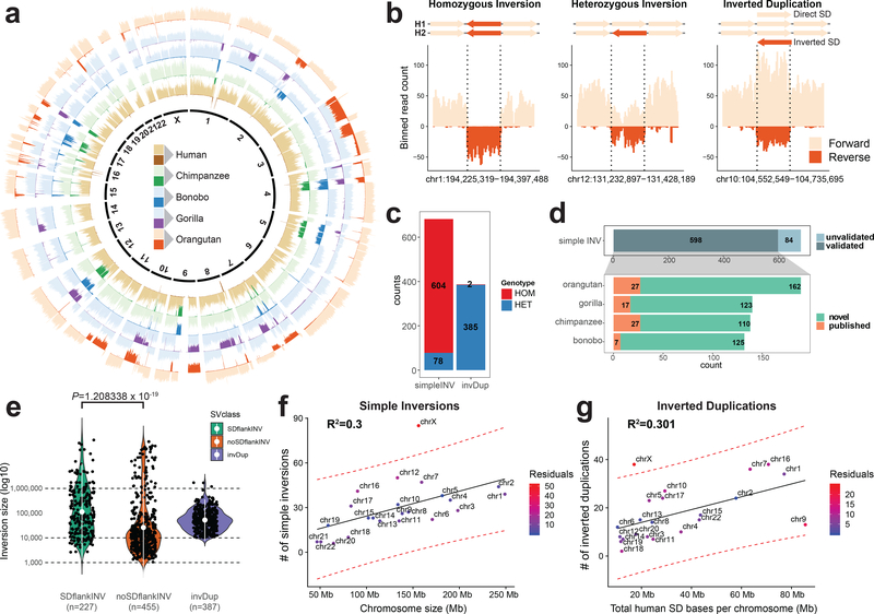
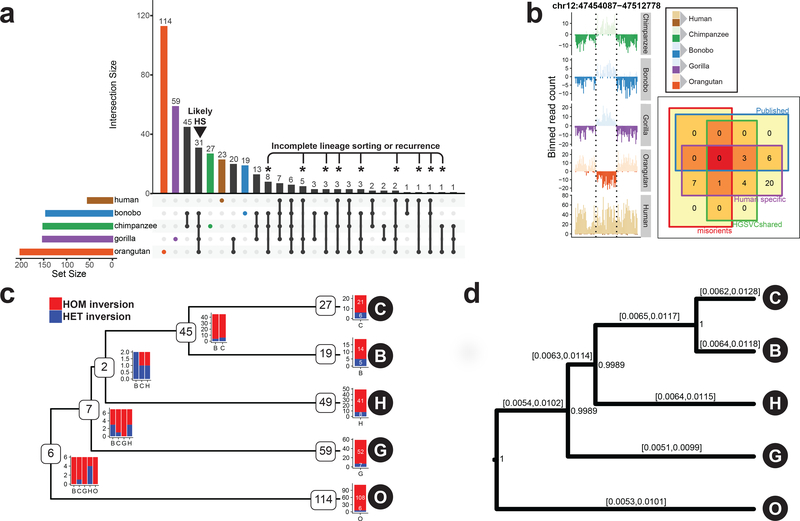
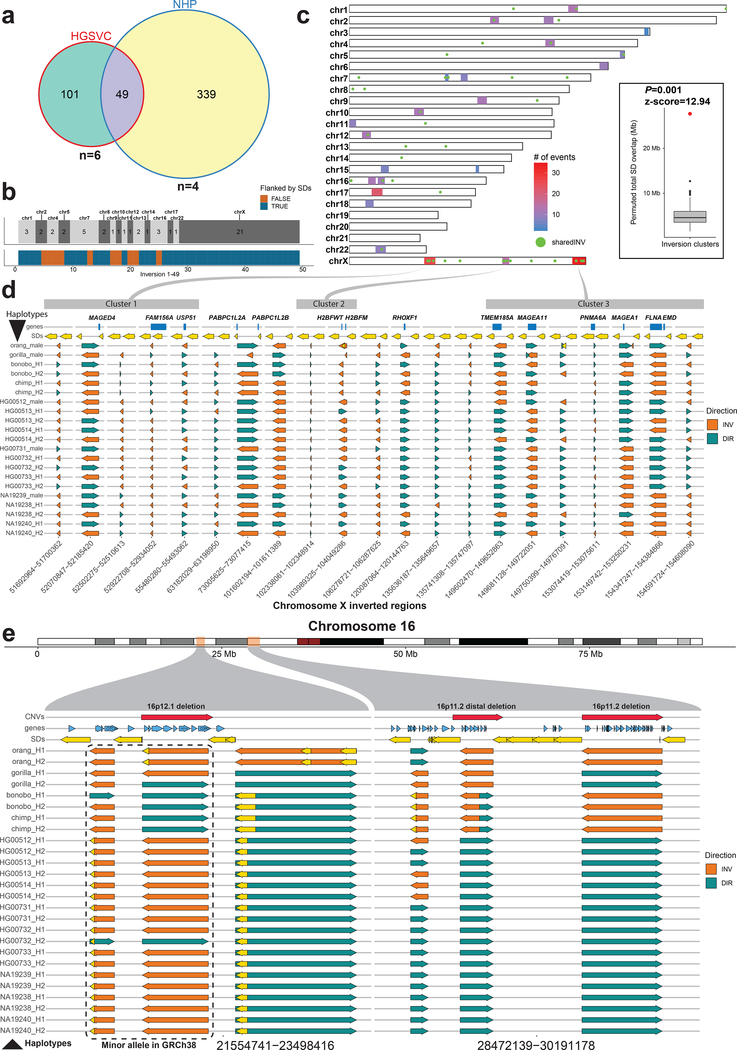
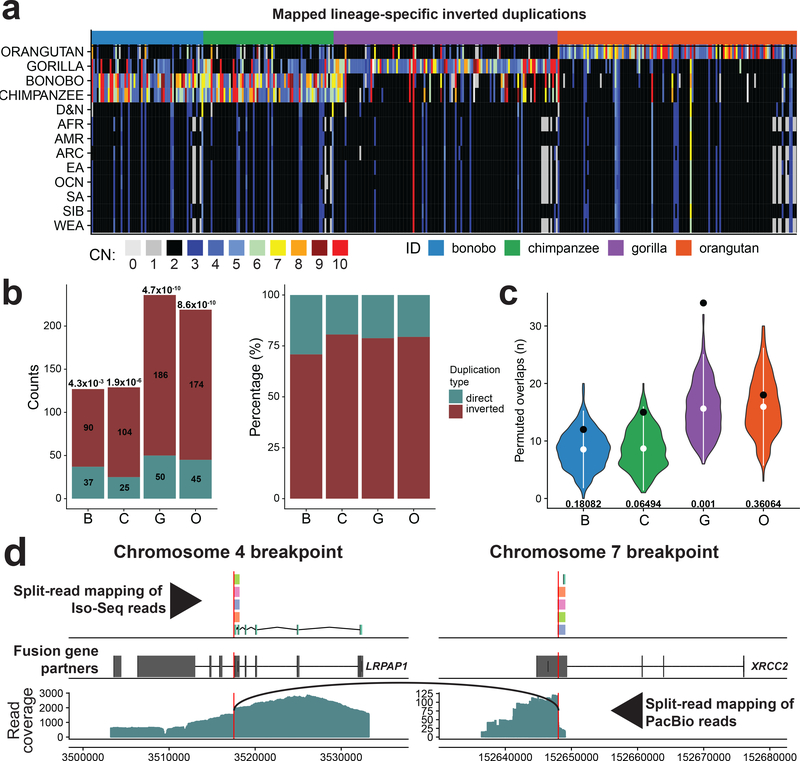
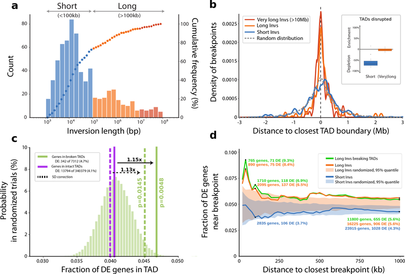
Inversions play an important role in disease and evolution but are difficult to characterize because their breakpoints map to large repeats. We increased by sixfold the number (n = 1,069) of previously reported great ape inversions by using single-cell DNA template strand and long-read sequencing. We find that the X chromosome is most enriched (2.5-fold) for inversions, on the basis of its size and duplication content. There is an excess of differentially expressed primate genes near the breakpoints of large (>100 kilobases (kb)) inversions but not smaller events. We show that when great ape lineage-specific duplications emerge, they preferentially (approximately 75%) occur in an inverted orientation compared to that at their ancestral locus. We construct megabase-pair scale haplotypes for individual chromosomes and identify 23 genomic regions that have recurrently toggled between a direct and an inverted state over 15 million years. The direct orientation is most frequently the derived state for human polymorphisms that predispose to recurrent copy number variants associated with neurodevelopmental disease.

Figure 1 |. Inversion call summary

a, Circular representation of composite files for each member of a great ape family. Genome of each individual is divided into 500-kb bins, and the number of reads mapped in forward (light color) and reverse (dark color) orientation in each bin is depicted as a bar along each chromosome. b, Example of inversion classes mapped in orangutan. Directional reads are binned into 10-kb bins (step 5 kb), and the number of reads mapped in forward (light color) and reverse (dark color) orientation is depicted as a vertical bar along a given genomic region. Inverted loci are highlighted by dashed lines. c, Summary of all inversions and inverted duplications mapped in this study. Inner circle summarizes the number of events found for each SV class (simple inversion, INV; inverted duplication, invDup). d, (i) Summary of validated simple inversions by other orthogonal technologies. (ii) Summary of validated simple inversions that appear to be novel in comparison to previously published data (green, novel; orange, published). e, Size distribution of simple inversions flanked by segmental duplications (SDs) (SDflankINV n = 227), simple inversions not flanked by SDs (noSDflankINV n = 455), and inverted duplications (invDup n = 387). White dot shows the mean of each distribution along with IQR range (Wilcoxon rank sum test). f, Scatterplot of the number of simple inversions (n = 682) given the chromosome length. g, Scatterplot showing the number of inverted duplications (n = 387) given the total length of known human SDs per chromosome. For f and g, regression line is added as a solid black line and 95% confidence intervals are highlighted as red dashed lines. Deviation from an expected number of inversions is expressed in the number of residuals.

Figure 2 |. Lineage-specific simple inversions and their evolutionary rates

a, An upsetR plot showing the number of shared inversions between members of the great ape family (≥50% reciprocal overlap). Black arrowhead points to putative human-specific inversions. Asterisks highlight inversions with recurrent or incomplete-lineage-sorting signatures. b, Example of a human-specific inversion predicted based on Strand-seq data. Inverted region is highlighted by dashed lines. Human-specific inversion is deemed as a region inverted in all NHPs in respect to the flanking region, but in direct orientation in humans. Inset: Venn diagram showing predicted human-specific inversions with respect to known genome minor alleles/misorients, human inversion polymorphisms, and already published human-specific inverted loci. c, A tree constructed based on shared simple inversions (≥50% reciprocal overlap) using hierarchical clustering. Each branching node contains a number of shared inversions in a given subtree together with a barplot showing inversion genotypes per individual (B, bonobo; C, chimpanzee; G, gorilla; H, human; O, orangutan). Tips of the tree contain the number of inversions without a significant overlap (<50%) with any other inversion and are likely species specific. Barplot showing inversion genotypes for such species-specific inversions is plotted at each tip of the tree (Methods). d, A rooted MCMC evolutionary tree constructed based on a nonredundant set of 358 autosomal simple inversions among great apes. Inversion rates are reported for each branch as 95% highest posterior density confidence intervals. Numbers at each branching node provide posterior support for this tree topology based on 10,000 MCMC trees sampled from an MCMC chain of 10,000,000 samples constructed from these data.

Figure 3 |. Shared inversions and inversion hotspots

a, Venn diagram showing overlapping simple inversions (50% reciprocal overlap) between HGSVC nonredundant dataset and NHP redundant dataset. b, Top tracks: number of shared inversions between HGSVC and NHP datasets from a shown as counts per chromosome. Bottom track: inversions flanked by segmental duplications (SDs) are colored blue and those not flanked are orange. c, A genome-wide map of detected inversion breakpoint clusters based on simple inversions from HGSVC and NHPs. A set of inversions (n = 49) from a is plotted over this genome-wide map as green dots. Inset: compares the total number of SD base pairs mapping to the 23 breakpoint clusters (red dot, observed = 29,138,268) compared to a random genome-wide simulation (n = 1,000 permutations, RegioneR ‘permTEST’, min: 1,653,112, 1stQ: 3,757,630, median: 5,301,424, 3rdQ: 7,084,019, max: 11,940,452). d, Each row represents a haplotype with all tested inversions phased along the whole X chromosome. Inverted direction is shown by an orange arrow and direct orientation by a teal arrow. Top track plots protein-coding genes (blue rectangles) that overlap with either the inversion itself or with flanking SDs, shown as yellow arrows. Previously defined inversion breakpoint clusters are shown as gray rectangles at the top of the figure and are linked to their location on chromosome X in c. e, Each row represents a haplotype with all tested inversions phased along the whole chromosome 16. Inverted direction is shown by an orange arrow and direct orientation by a teal arrow. Top track plots protein-coding genes (blue arrows) that overlap either the inversion itself or with a flanking SD, shown as yellow arrows. Previously published pathogenic CNVs are shown as red arrows in the top track.

Figure 4 |. Evolutionary impact of inverted duplications

a, Heatmap of estimated copy number (mean CN) per inverted duplication (columns) in multiple human populations and NHPs (rows). b, Left: number of mapped duplicated regions in inverted versus direct orientation. Significance of observed differences between inverted and direct duplications is reported above each bar as P-value (chi-squared with Bonferroni correction). Right: each bar shows the proportions of inverted and direct duplications per NHP (colored as denoted in a). c, Enrichment analysis of inverted duplication in 0.05 fraction of each chromosome end (1–22 and X). Observed counts are shown by a black dot and the distributions of permuted counts (n = 1,000 permutations, RegioneR ‘permTEST’,) are depicted by violin plots. White dots show the mean of each distribution (B-8.54, C-8.69, G-15.6, O-16). At the bottom of each distribution there is a P-value showing the significance of difference between observed (B-12, C-15 G-34 O-18) and permuted counts. d, Predicted gene fusion between XRCC2 on chromosome 7 and LRPAP1 on chromosome 4. Upper track: split-read mappings of Iso-Seq reads over the predicted breakpoint (red vertical line). Iso-Seq reads that belong to the same transcript share the same color. Middle track: gene models of above mentioned genes (Exons, wide boxes; Introns, lines in between). Bottom track: split-read mapping of PacBio reads over the fusion breakpoint on chromosome 4. Black arc line connects ends of PacBio reads with split-read mappings.

Figure 5 |. Impact of copy-neutral inversions on genome topology and differential gene expression

a, Length distribution of all 387 nonredundant simple inversions, classified as ‘Short’ (<100 kb; blue) or ‘Long’ (>100 kb, orange). The histogram illustrates absolute counts of binned inversion lengths and the overlaid dots represent the cumulative frequency of inversions corresponding to each bin. (bp, base pair; kb, kilobase). b, Distance of each inversion breakpoint (centered at 0) to the closest topologically associating domain (TAD) boundary, stratified by inversion length (color coding according to a). The expected distance distribution for randomly placed breakpoints is indicated by the gray dotted line (Mb, Megabase). The inlay displays the proportion of inversions (stratified by length) that disrupt TADs (median short: −67.1%, median long: −2.4%). Percent ‘enrichment’ or ‘depletion’ is shown as the ratio of observed over expected disruptions calculated after randomizing inversion locations (Methods). c, Proportion of differentially expressed (DE) genes in TADs classified as either ‘broken’ (solid green horizontal line) or ‘intact’ (solid purple horizontal line). The underlying histogram depicts the expected DE frequency after randomizing TAD labels. Dotted lines represent the DE proportion after excluding genes in segmental duplications (SDs). One-sided permutation testing was used to derive P-values (Methods). d, Proportion of DE genes relative to inversion breakpoints and stratified by inversion length or whether the inversion disrupts a TAD. The shaded areas show the expected DE proportion measured in matched randomized breakpoints.

References

1. Sturtevant AH Genetic factors affecting the strength of linkage in Drosophila. Proc. Natl. Acad. Sci. U. S. A 3, 555–558 (1917). - PMC - PubMed
1. Antonacci F et al. Characterization of six human disease-associated inversion polymorphisms. Hum. Mol. Genet 18, 2555–2566 (2009). - PMC - PubMed
1. Chaisson MJP, Wilson RK & Eichler EE Genetic variation and the de novo assembly of human genomes. Nat. Rev. Genet 16, 627–640 (2015). - PMC - PubMed
1. Chaisson MJP et al. Multi-platform discovery of haplotype-resolved structural variation in human genomes. Nat. Commun 10, 1784 (2019). - PMC - PubMed
1. Kidd JM et al. Mapping and sequencing of structural variation from eight human genomes. Nature 453, 56–64 (2008). - PMC - PubMed
Publication types