Spatial planning with long visual range benefits escape from visual predators in complex naturalistic environments

Abstract

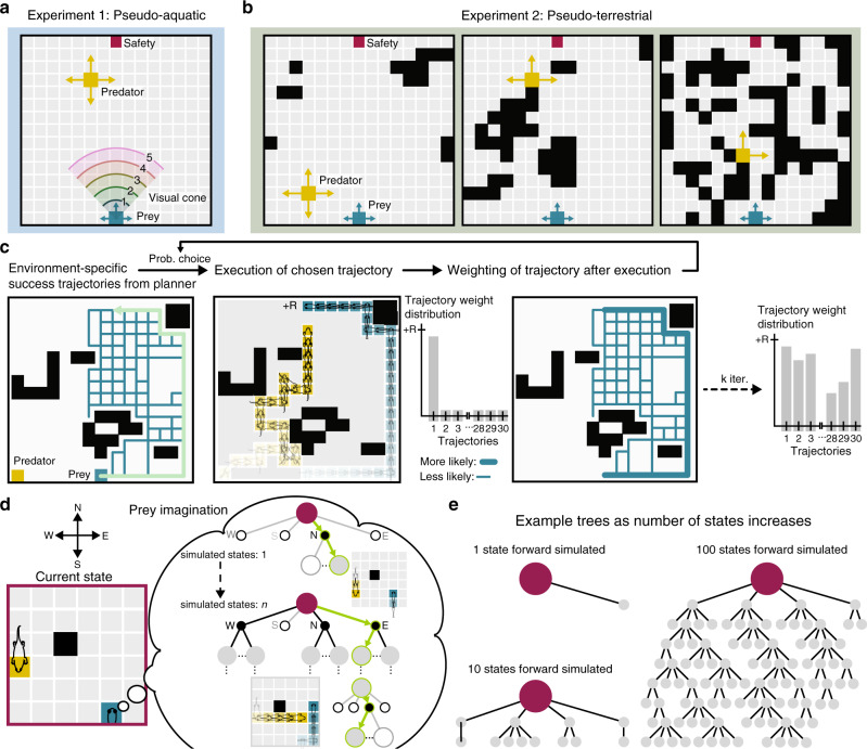
It is uncontroversial that land animals have more elaborated cognitive abilities than their aquatic counterparts such as fish. Yet there is no apparent a-priori reason for this. A key cognitive faculty is planning. We show that in visually guided predator-prey interactions, planning provides a significant advantage, but only on land. During animal evolution, the water-to-land transition resulted in a massive increase in visual range. Simulations of behavior identify a specific type of terrestrial habitat, clustered open and closed areas (savanna-like), where the advantage of planning peaks. Our computational experiments demonstrate how this patchy terrestrial structure, in combination with enhanced visual range, can reveal and hide agents as a function of their movement and create a selective benefit for imagining, evaluating, and selecting among possible future scenarios-in short, for planning. The vertebrate invasion of land may have been an important step in their cognitive evolution.

Fig. 1. Environment models and schematic of habit- and plan-based action selection.

a, b Example 2-D environments used in the simulations; black squares represent obstacles. Examples of low, medium, and high clutter are shown for the pseudo-terrestrial condition. These environments can be experienced in the context of a predator-prey online game at https://maciverlab.github.io/plangame/. c Schematic of habit. A set of success paths (initially all weighted equally) are used in a loop in which a path is selected (green line with arrow) with probability proportional to its weight. After execution, the path is weighted by its total discounted reward, provided that it resulted in survival. Example weight distribution after k trials. d Schematic of planning. The prey imagines a tree of possibilities from the current state (dark red) by selecting virtual actions (green: next action and next state, white fill and black edge: unexplored possible actions, white fill and gray edge: unexplored possible next states, black fill: explored actions, gray fill: explored next states). Example virtual actions by the prey and the predator are shown on the smaller grid. e Example trees grown given a specified number of states being forward simulated.

Fig. 2. The utility of different behavioral controllers in open environments.

a Prey survival rate in pseudo-aquatic environments (Fig. 1a). The line plot shows the mean survival rate, and the surrounding fill indicates  ±s.e.m across random initial predator locations (n = 20). Two-tailed Kruskal–Wallis (KW) test: H₁₀₀ = 2.0, p = 0.57; H₁₀₀₀ = 55.5, p < 10⁻¹⁰; H₅₀₀₀ = 81.3, p < 10⁻¹⁶. b Mean change in survival rate across all the planning levels shown in (a) (see Methods). Horizontal line: mean; Shaded region:  ±s.e.m; Box: 95% confidence interval of the mean; Vertical line: range of the data. n = 20 independent random initial predator locations. Mann–Whitney U (MWU) tests (two-tailed) across visual ranges (with Bonferroni correction: U_1,2 = 54.0, U_2,3 = 159.5, U_3,4 = 127.5, and U_4,5 = 63.0 (***p < 0.0001; n.s. is not significant p > 0.025) (KW over all visual ranges H = 55.4, p < 10⁻¹⁰). c Heatmaps of all action sequences taken by the prey that resulted in prey survival at the maximum planning level (5000 states), with color density proportional to frequency. Color bar action frequencies range from 1 to 206, dependent on visual range (for all paths see Supplementary Fig. 3). Survival paths are aggregated across all tested predator locations (n = 20) and the total number of episodes per predator location (n = 100). d Mean ± s.e.m. across random initial predator locations (n = 20) of survival rate for prey that uses habit (red dashed line). The planning data (blue solid line) is another representation of the plot shown in (a) at maximum planning level (±s.e.m across random initial predator locations; n = 20). KW test (two-tailed) for each visual range (with Bonferroni correction): H₁ = 0.11, p₁ = 0.74; H₂ = 3.53, p₂ = 0.30; H₃ = 4.26, p₃ = 0.20; H₄ = 3.42, p₄ = 0.32; H₅ = 4.04, p₅ = 0.22. Source data are provided as a Source Data file.

Fig. 3. The utility of different behavioral controllers in habitats with varying complexity.

a Mean survival rate versus clutter density across random predator locations (n = 5), for a given planning level. The fill indicates  ±s.e.m. across randomly generated environments (n = 20). b Mean change in survival rate across all planning levels shown in (a) calculated for Low: 0.0–0.3 entropy; Mid 0.4–0.6; High 0.7–0.9. Horizontal line: mean; Shaded region:  ±s.e.m; Box: 95% confidence interval of the mean; Vertical line: range of the data. n = 20 for each entropy level; mean change in survival rate is averaged across tested initial predator locations (n = 5) and across entropy grouping. MWU tests (two-tailed) across entropy groupings (with Bonferroni correction): U_low,mid = 39.0, U_mid,high = 51.0, and U_low,high = 142.0, (***p < 10⁻⁴; n.s. is not significant p = 0.06). (KW across entropy ranges H = 24.7, p < 10⁻⁵). c Spatial complexity with respect to entropy. The line plot shows the mean complexity and the interquartile range (n = 20 generated environments). Insert shows example 4 × 4 environments and their corresponding visibility networks. d–g Heatmaps of all action sequences taken by the prey that resulted in prey survival at the maximum planning level (5000 states) in four out of the 200 environments examined, with color density proportional to frequency. Color bar action frequencies range from 1 to 68, dependent on entropy level. Survival paths are aggregated across all tested predator locations (n = 5) and total number of episodes (n = 50). For other examples see Supplementary Fig. 5. h Path spread denotes the percent of unique cells occupied by successful action sequences at the 5000 state planning level. Plot representation, and low, mid, and high entropy ranges as in (b) (n_low = 76, n_mid = 58, and n_high = 46 generated environments). MWU tests (two-tailed) across entropy groupings (with Bonferroni correction): U_low,mid = 1109.0, U_mid,high = 246.0, and U_low,high = 595.0 (***p < 10⁻⁷). i Graph distance between action sequences that resulted in prey survival implemented by habit. Plot representation, and low, mid, and high entropy ranges as in (b) (n_low = 70, n_mid = 41, and n_high = 32 generated environments). MWU tests (two-tailed) across entropy groupings (with Bonferroni correction): U_low,mid = 1069.0, U_mid,high = 322.0, and U_low,high = 717.0 (*p = 0.013; **p = 0.002; ***p = 0.0001). j Mean survival rate for prey that uses habit (red dashed line). Representation as in (a). The planning data (blue solid line) as in (a) (±s.e.m. across randomly generated environments (n = 20), averaged across random initial predator locations (n = 5)). KW tests (two-tailed) for survival rate under habit- and plan-based action selection: low entropy (0.0–0.3) p > 0.05; mid entropy (0.4–0.6) p < 10⁻⁴; high entropy (0.7–0.9) p > 0.05. Source data are provided as a Source Data file.

Fig. 4. Using spatial connectivity to arbitrate between behavioral controllers.

a Heatmap of all predator paths that resulted in prey capture. Color bar: 1–87. b Eigencentrality of an open environment overlaid with representative prey success paths in teal, and prey capture (see (a)) in orange. Line thickness proportional to action frequency. c Multiple-T maze overlaid with eigencentrality and eigencentrality gradient. Color density proportional to the eigencentrality and eigencentrality gradient of each cell of the quantized maze. Johnson and Redish showed that the neural representation of place (reconstruction on the right) moved ahead of the animal while it paused at the choice point. d Example environments (top row entropy = 0.5, bottom row entropy = 0.9) and their eigencentralities and eigencentrality gradients (see Supplementary Fig. 9 for prey success paths). Transition regions (red box) from low to high eigencentrality and behavioral control based on change in gradient and value of eigencentrality (see Supplementary Fig. 10 for other transition region examples). e Mean spatial autocorrelation (global Moran's I) of the environment eigencentrality. Horizontal line: mean; Shaded region:  ±s.e.m; Box: 95% confidence interval of the mean; Vertical line: range of the data. For all entropy levels n = 20. MWU tests (two-tailed) across entropy groupings (with Bonferroni correction): U_low,mid = 15.0, U_mid,high = 13.0, and U_low,high = 178.0, (***p < 10⁻⁶; n.s. is not significant p = 0.28). f Average percent time spent in decision making regime (habit vs planning) when environments are grouped based on their spatial autocorrelation of eigencentrality (n_low = 50: bottom 25%, n_high = 46: top 75%). The error bars indicate  ±s.e.m of percent time spent. g Survival rate for a prey that uses planning (blue), habit (red), and hybrid control (purple) based on environment eigencentrality (see (d); see Methods). Environment grouping as in (f) (n_low = 50, and n_high = 46), and representation as in (e). Two-tailed KW test for survival rate in environments with low eigencentraliy clustering H = 0.952, p = 0.62. Two-tailed MWU test with Bonferroni correction for survival rate under hybrid and plan-based action selection in environments with high eigencentrality clustering U = 820.5, p = 0.09. Source data are provided as a Source Data file.

Fig. 5. Comparison of generated environments to natural habitats.

a Distribution of lacunarities of generated environments (see Supplementary Methods 1). The line plot shows the mean natural log of average lacunarity (see Methods) and the interquartile range (n = 20 at each entropy level). Coastal: blue line ≥1.16, n_coastal = 70; Land: green line 0.23–1.34, n_land = 139; Structured Aquatic: pink line 0.03–0.41, n_{structured aquatic} = 42 (Supplementary Table 1). The green circle highlights a zone of lacunarity where planning outstrips habit (based on Fig. 3j). Insert shows an example image from the Okavango Delta in Botswana (≈800 m × 800 m, from Google Earth), and its average lacunarity (ln(Λ_avg)). The Okavango is considered a modern analogue of the habitats that early hominins lived within after branching from chimpanzees. For additional images and their corresponding lacunarity plots see Supplementary Fig. 11. b Spatial complexity (see Fig. 3c) of generated environments grouped by natural environment bands. Horizontal line: mean; Shaded region:  ±s.e.m; Box: 95% confidence interval of the mean; Vertical line: range of the data (n_coastal = 70, n_land = 134, n_{structured aquatic} = 41 generated environments). MWU tests (two-tailed) across environment groupings (with Bonferroni correction): U_coastal,land = 2103.5, U_{land, structured aquatic} = 666.5, and U_{coastal,structured aquatic} = 1405.0, (***p < 10⁻¹⁰; n.s. is not significant p = 0.43). c The incremental benefit of planning (see Fig. 3b) of generated environments grouped by natural environment bands. Plot representation as in (c). (n_coastal = 70, n_land = 139, n_{structured aquatic} = 42 generated environments). MWU tests (two-tailed) across environment groupings (with Bonferroni correction): U_coastal,land = 3631.0, U_{land, structured aquatic} = 2001.0, and U_{coastal,structured aquatic} = 1263.5, (**p = 0.001; ***p = 0.001; n.s. is not significant p = 0.08). d Survival rate for a prey that uses planning (blue) and habit (red) of generated environments grouped by natural environment bands. Plot representation as in (b). (n_coastal = 70, n_land = 139, n_{structured aquatic} = 42 generated environments). KW tests (two-tailed) for survival rate under habit- and plan-based action selection: H_coastal = 3.29, p = 0.07; H_land = 40.7, p < 10⁻⁹; H_{structured aquatic} = 1.16, p = 0.3. In (b), (c), and (d) black dot and vertical bar overlay indicates mean ± s.e.m. of the variable of interest in environments where planning outperforms habit (green shaded region in (a)). Source data are provided as a Source Data file.

References

1. MacIver MA, Schmitz L, Mugan U, Murphey TD, Mobley CD. Massive increase in visual range preceded the origin of terrestrial vertebrates. Proc. Natl Acad. Sci. USA. 2017;114:E2375–E2384. - PMC - PubMed
1. Keramati M, Smittenaar P, Dolan RJ, Dayan P. Adaptive integration of habits into depth-limited planning defines a habitual-goal–spectrum. Proc. Natl Acad. Sci. USA. 2016;113:12868–12873. - PMC - PubMed
1. Stein, W. E. et al. Mid-Devonian Archaeopteris roots signal revolutionary change in earliest fossil forests. Curr. Biol. 0 (2019). - PubMed
1. Yamakita T, Miyashita V. In Integrative Observations and Assessments, Ecological Research Monographs. Tokyo: Springer Japan; 2014. pp. 131–148.
1. Daw ND, Niv Y, Dayan P. Uncertainty-based competition between prefrontal and dorsolateral striatal systems for behavioral control. Nat. Neurosci. 2005;8:1704–1711. - PubMed
Publication types