A Slow Short-Term Depression at Purkinje to Deep Cerebellar Nuclear Neuron Synapses Supports Gain-Control and Linear Encoding over Second-Long Time Windows

Abstract

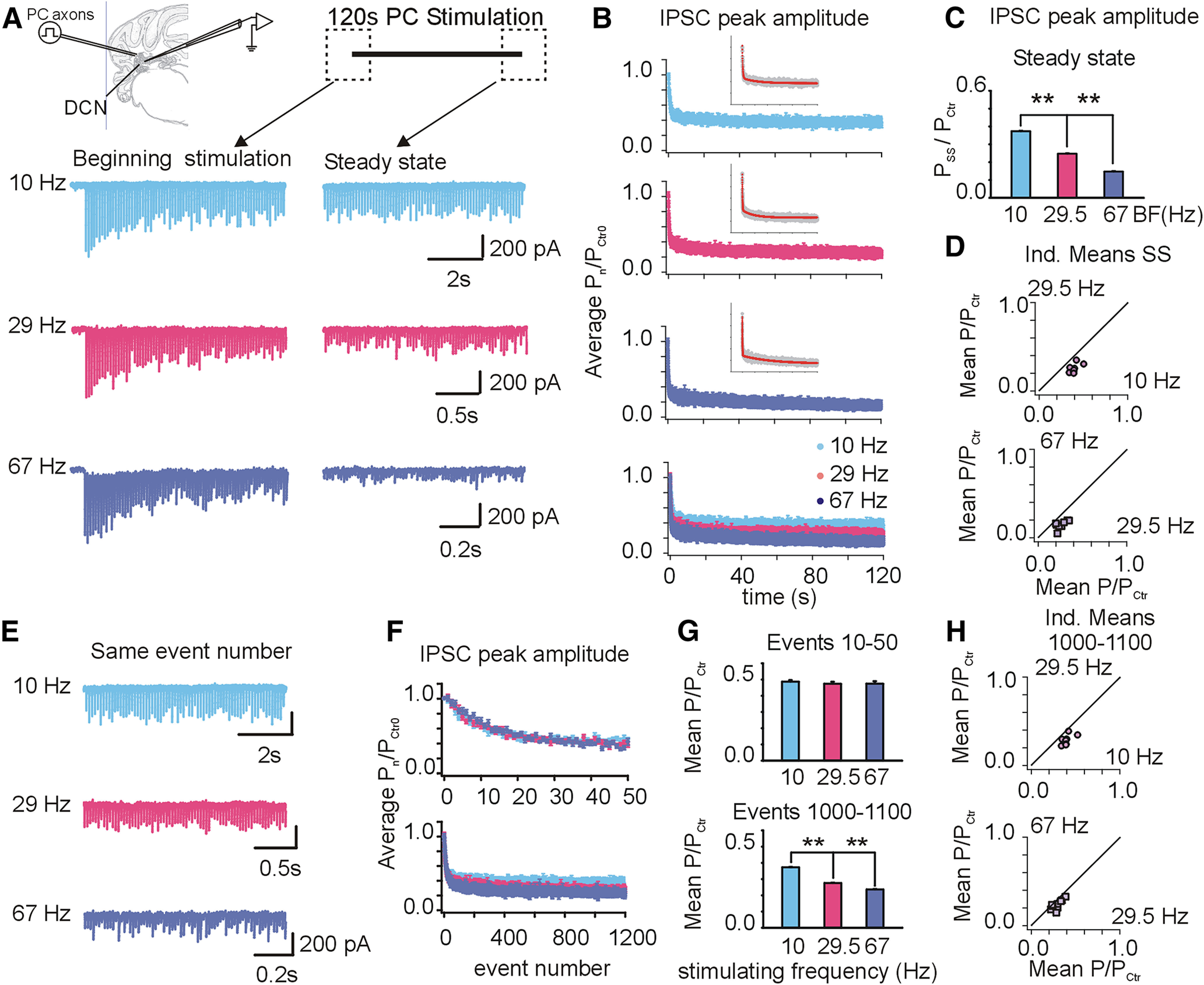
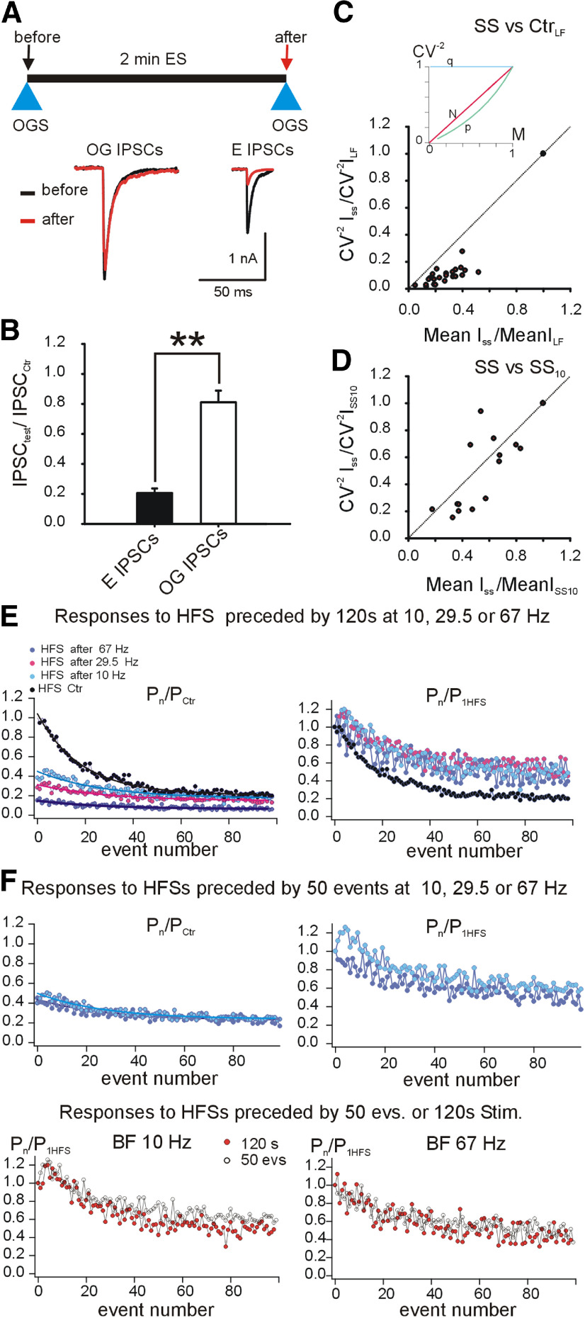
Modifications in the sensitivity of neural elements allow the brain to adapt its functions to varying demands. Frequency-dependent short-term synaptic depression (STD) provides a dynamic gain-control mechanism enabling adaptation to different background conditions alongside enhanced sensitivity to input-driven changes in activity. In contrast, synapses displaying frequency-invariant transmission can faithfully transfer ongoing presynaptic rates enabling linear processing, deemed critical for many functions. However, rigid frequency-invariant transmission may lead to runaway dynamics and low sensitivity to changes in rate. Here, I investigated the Purkinje cell to deep cerebellar nuclei neuron synapses (PC_DCNs), which display frequency invariance, and yet, PCs maintain background activity at disparate rates, even at rest. Using protracted PC_DCN activation (120 s) to mimic background activity in cerebellar slices from mature mice of both sexes, I identified a previously unrecognized, frequency-dependent, slow STD (S-STD), adapting IPSC amplitudes in tens of seconds to minutes. However, after changes in activation rates, over a behavior-relevant second-long time window, S-STD enabled scaled linear encoding of PC rates in synaptic charge transfer and DCN spiking activity. Combined electrophysiology, optogenetics, and statistical analysis suggested that S-STD mechanism is input-specific, involving decreased ready-to-release quanta, and distinct from faster short-term plasticity (f-STP). Accordingly, an S-STD component with a scaling effect (i.e., activity-dependent release sites inactivation), extending a model explaining PC_DCN release on shorter timescales using balanced f-STP, reproduced the experimental results. Thus, these results elucidates a novel slow gain-control mechanism able to support linear transfer of behavior-driven/learned PC rates concurrently with background activity adaptation, and furthermore, provides an alternative pathway to refine PC output.SIGNIFICANCE STATEMENT The brain can adapt to varying demands by dynamically changing the gain of its synapses; however, some tasks require ongoing linear transfer of presynaptic rates, seemingly incompatible with nonlinear gain adaptation. Here, I report a novel slow gain-control mechanism enabling scaled linear encoding of presynaptic rates over behavior-relevant time windows, and adaptation to background activity at the Purkinje to deep cerebellar nuclear neurons synapses (PC_DCNs). A previously unrecognized PC_DCNs slow and frequency-dependent short-term synaptic depression (S-STD) mediates this process. Experimental evidence and simulations suggested that scaled linear encoding emerges from the combination of S-STD slow dynamics and frequency-invariant transmission at faster timescales. These results demonstrate a mechanism reconciling rate code with background activity adaptation and suitable for flexibly tuning PCs output via background activity modulation.

Keywords: background activity; gain modulation; short-term memory; short-term plasticity; sustained activity; synaptic transmission.

Figure 1.

Protracted PC stimulation unveils an S-STD. A, Top, Sketch of experimental configuration and stimulation paradigm. Bottom, Typical examples of IPSCs from the same neuron evoked by 2 min trains of stimuli applied to PC axons at the frequencies (BF) indicated on the left, at the beginning (left), and at the end of stimulation (right). Note the different time scales. B, Top to bottom, Mean normalized IPSC peak amplitude as a function of time for BFs 10 Hz (light blue, n = 11), 29.5 Hz (red, n = 9), and 67 Hz (dark blue, n = 9), and all three plots overlaid (symbols represent mean ± SEM) illustrate two phases of decay. Color code applies to all figures, unless otherwise stated. The double exponential decay fits in the insets: fast tau: 0.81 ± 0.04, 0.41 ± 0.012, and 0.33 ± 0.007 s and slow tau: 23 ± 1.9, 18 ± 0.5, and 47 ± 1.2 s for 10, 29.5, and 67 Hz BFs, respectively. C, Average normalized steady-state phasic IPSCs amplitude (IPSC_SS) versus BF (averages calculated over the last 100 events of the data plotted in B; 0.37 ± 0.002, 0.25 ± 0.002, and 0.15 ± 0.002 for 10, 29.5, and 67 Hz BFs, respectively: 10 versus 29.5 Hz [Mann–Whitney rank sum test] and 29.5 vs 67 Hz [t test], p < 0.001 for both comparisons). D, Results from individual neurons illustrate decreasing mean IPSC_SS with increasing BF (averages over 100 events). Top, IPSC amplitude for 29.5 versus 10 Hz. Bottom, IPSC amplitude for 67 versus 29.5 Hz. All points fall below the unity line. E, Typical examples from the same neuron in A of IPSCs evoked by the same ordinal stimuli but at different BFs (indicated on the left). The 10 Hz trace is the same shown in A for comparison. F, Summary of IPSC amplitude as in B, but as a function of the event number (color labeled as B). Top, Events 1-50. Bottom, Events 1-1200. G, Averages as in C, calculated over the events indicated on top of each bar plot. Top, Events 10-50: 0.49 ± 0.01, 0.47 ± 0.02, and 0.47 ± 0.03, for 10, 29.5, and 67 Hz, respectively; Wilcoxon signed rank sum test: 10 versus 29.5 Hz, p = 0.115; 29.5 versus 67 Hz, p = 0.7. Bottom, Events 1000-1100: 0.37 ± 0.002, 0.276 ± 0.002, and 0.236 ± 0.002, for 10, 29.5, and 67 Hz, respectively, t test, 10 versus 29.5 and 29.5 versus 67 Hz, p < 0.001 for both. H, Similar as in D, but for mean IPSCs amplitudes calculated over stimuli 1000-1100th for each neuron. Top, 29.5 Hz versus 10 Hz. Bottom, 67 versus 29.5 Hz. Data are mean ± SEM. **p < 0.001.

Figure 2.

S-STD frequency dependence under irregular activation patterns and in DCNs from adult mice. A, Top, Representative traces of IPSCs evoked in the same neuron by 2 min Poisson-like stimulation at the mean frequencies indicated on the left. Bottom, Summary plots of mean IPSCs amplitudes calculated over the stimuli indicated on top of each graph as in Figure 1, but for Poisson-like stimulation at 10 Hz (n = 9) and 70 Hz (n = 7). Significance assessed using Mann–Whitney rank sum test (0.33 ± 0.002, 0.23 ± 0.003 for 10 and 70 Hz, for events 1000-1100th; and 0.33 ± 0.002, 0.15 ± 0.003 for 10 and 70 Hz, respectively, for steady-state IPSCs, p < 0.001). B, Left, Normalized average amplitude as a function of event number of PC_DCN IPSC recordings obtained from slices from P55-P72 animals (BF 10 Hz, n = 8, BF 67 Hz, n = 7). Right, Summary plots of mean IPSC amplitudes calculated from the graphs on the left, over the events indicated on top of each bar plot (1000-1100th for 10 and 67 Hz BFs: 0.45 ± 0.002 and 0.32 ± 0.002, t test, p < 0.001; average of 100 events at steady state: 0.45 ± 0.002 and 0.26 ± 0.003 for 10 and 67 Hz, respectively, t test, p < 0.001). **p < 0.001.

Figure 3.

PC background activity modulates the DCN synaptic and spiking responses to HFS trains. A, Top, Stimulation paradigm. Bottom, Mean charge transfer amplitude during HFS (100 events, 180 Hz), normalized to that of control IPSCs as a function of prior BF. B, Typical examples from two different neurons illustrating how prior BF (indicate on the left of each trace) modulates the amplitude of IPSCs evoked by the HFS (indicated by the gray box). C, Four typical examples of DCN cell-attached recordings used to investigate how BF modulates the suppression of DCN spontaneous firing rate induced by HFSs delivered after protracted stimulation at 10 Hz (left) or at 67 Hz (right). Each row corresponds to the same neuron. Vertical line indicates the occurrence of one spike. D, Scatter plot of changes in DCN firing rate induced by HFSs (HFS-Basal rate), for HFS preceded by BF 67 Hz versus HFSs preceded by BF 10 Hz. All points fall below the unity lines (diagonal), indicating stronger inhibition after BF 10 Hz. Inset, Mean values and SEM for BF 10 and 67 Hz. E, Effect of nonstationary BF stimulation on HFSs suppression of DCN rate. Top, Stimulation paradigm. Bottom, Mean HFS-induced changes in DCN firing rate as a function of the 67 Hz train duration, normalized to the responses evoked without switch to 67 Hz (top, dashed line, 100%). Bottom, Dashed line indicates the value of mean responses to HFS after 120 s at 67 Hz only. The data were fitted with a single exponential function (R² = 0.99, n = 6). F, Same as in E, but for a switch in BF from 120 s at 67 Hz to 10 Hz (R² = 0.94, n = 6). **p < 0.001, *p < 0.05.

Figure 4.

Linear PC_DCN transfer function of subsecond changes in PC rate with gain dependent on preceding BF. A, Top, Stimulation paradigm to investigate changes in PC_DCN input/output gain: 0.5 s test trains of stimuli at different frequencies (from 10 to 260 Hz) delivered after 120 s of stimulation at different BFs (0, 10, 29.5, or 67 Hz). Bottom, Summary of measured PC_DCN synaptic charge transfer during the test trains (Q _TEST), normalized to the charge transfer of corresponding control IPSCs (Q P_Ctrl), expressed per time unit, as a function of the test frequency. The plots corresponding to test trains applied from rest (0 Hz), or after 120 s at 10, 29.5, or 67 Hz are labeled on the right of each curve (color code as before). Note the almost linear relationship between 10 and 180 Hz and the different slopes for different BFs, indicative of different gains (gain of linear fits from 10 to 200 Hz: 0.34 ± 0.002, 0.23 ± 0.001, and 0.085 ± 0.004 for 10, 29.5, and 67 Hz, respectively). Dashed black line (unity line) indicates the expected values for nondepressing/nonfacilitating PSCs. B, Plots of changes in DCN firing rate (difference to steady state rate) as a function of the test train frequency from experiments using the same stimulation paradigm as in A, and DCN cell-attached recordings. Top, Two typical examples exhibit approximately linear relationships (lines correspond to linear fits to the data). Left, bottom, One unit exhibited nonlinear relationship after 10 Hz BF (points linked by straight lines). Right, bottom, Average changes in DCN firing rate from neurons with linear relationship (n = 6, lines correspond to linear fits; gain: −0.34 ± 0.005 and −0.22 ± 0.012 Hz/Hz and R² = 0.999 and 0.997 for 10 and 67 Hz BF, respectively). C, Scatter plots of gains (estimated by the slopes of linear fits as in B) for BF 67 Hz versus their corresponding values for BF 10 Hz (n = 6) for single neurons (Wilcoxon sign rank test, p = 0.031, n = 6; diagonal is the unity line). D, Same data from A, but normalized to the charge transferred by the corresponding IPSCs at steady state (Q P_SS). The responses to test stimuli applied from rest, 0 Hz, in empty black. The plots corresponding to different BFs overlap around the unity line indicating that the synaptic strength at steady state determines the BF-dependent gains (i.e., the slopes shown in A). Linear fits for the test frequency range 10-200 Hz (for clarity not shown). For BF 10 Hz: slope 1.0 ± 0.04, R² = 0.99; BF 29.5 Hz: slope 1.1 ± 0.06, R² = 0.99; BF 67 Hz: slope 0.9 ± 0.03, R² = 0.99. Dashed line indicates unity line. Inset, same plot as in A overlaid to colored dashed lines indicating the result of multiplying the corresponding mean Q P_ss by the test train frequency, for each BF. E, Average charge transfer amplitude for IPSCs at steady state normalized to control IPSCs (Q P_ss) as a function of the BF (n = 25). Curve indicates the fit with a rational function (n = 25, R² = 0.999). Inset, Averaged measured charge transfer amplitude at steady state per time unit, normalized to control IPSCs (Q ss) versus the BF (note different scale). F, Same as in D, but for the first 100 ms of the responses to the 500 ms test trains show gain > 1.

Figure 5.

Exploration of S-STD mechanism. A, Combined OG and ES to explore input specificity. Top, Experimental paradigm. Bottom, Representative examples of OG IPSCs and ES IPSCs before (control, black) and after (test, red) 2 min ES at 67 Hz. B, Plot showing significant differences in average OG and ES IPSC amplitudes after 2 min ES at 67 Hz (normalized to the corresponding controls: IPSCs induced after 2 min without ES; 0.81 ± 0.078 and 0.21 ± 0.03 for OG and ES IPSCs, respectively, paired t test, p < 0.001, n = 8) suggests input specificity. C, Plot of CV⁻² versus their corresponding mean amplitudes (M) for IPSCs depressed to steady state steady using 120 s stimulation at 10, 29.5, or 67 Hz, normalized to the values of their corresponding control IPSCs (n = 8). Inset, Expected CV⁻² versus M values for changes in the parameters N (red line), p (green), or q (blue) of a binomial release model. D, Same as in C, but for IPSCs depressed using BF 29.5 or 67 Hz normalized the corresponding BF 10 Hz values (n = 7). Dashed line indicates unity line. Fit of data using a linear function (R² = 0.78, slope 1.07 ± 0.13, n = 7; data not shown). E, Left, Plot of mean IPSC peak amplitude normalized to control IPSCs as a function of the HFS event number for HFSs (100 events, 180 Hz) applied from rest (black, n = 17) or after 120 s of stimulation at 10 Hz (light blue, n = 11), 29.5 Hz (red, n = 9), and 67 Hz (dark blue, n = 9). Continuous lines indicate exponential fits to the curves. Note the faster decay for the HFS applied from rest but similar slower values for the other curves, suggesting similar probability of release after the first events. Right, Plot of IPSC peak amplitudes normalized to the value of the first IPSC of the HFS, illustrates relative facilitation during the first events for BFs 10 and 30 Hz, but similar decay rate and percentage of decay for different BFs afterward. F, Left, Same as in E (left), but for HFSs applied after 50 events at 10 or 67 Hz (color code as in E). Note the relative facilitation of the first events for BF 10 Hz, but similar degree of depression at the end of the HFS for 10 and 67 Hz BF. Continuous lines indicate exponential fits. The data correspond to a different set of neurons than those shown in E. Right, Same data as on the left, but normalized to the corresponding first IPSC of the HFS. Bottom, Plots represent superimposed mean IPSC amplitude normalized to the first HFS event for HFSs delivered after 120 s of stimulation (red circles) or 50 events (empty circles) after BF 10 Hz (left) or 67 Hz (right) as a function of the HFS event number. The similarity in the IPSC amplitude time course after 120 s or 50 events suggests that S-STD did not alter the relative proportion of fast synaptic facilitation and depression evoked by the HFSs. **p < 0.001.

Figure 6.

Experimental and simulated responses of a two-pool and facilitation model of PC_DCNs to different BFs. A, Top, D + F model scheme. Synapses contain two different pools of vesicles A and B, which differ in release probability (Pr), time constant of recovery (Tau_R), and presence of facilitation. Bottom, The predicted output of a two-pool and facilitation model (D + F model) explains the experimental responses to the first 100 events of stimulation trains at 10, 29.5, and 67 Hz (same data as in Fig. 1). B, Detail of the model responses to the first 8 events of the trains at 10 and 67 Hz using a semilogarithmic plot to illustrate slower decaying rates with higher stimulating frequencies. C, Left and right plots (for 10 and 67 Hz stimulation rates, respectively) represent, from top to bottom, the data (circles) and model output (continuous lines), the predicted IPSC amplitudes for Pools A and B (PA, PB, red and blue), and the size of the ready to be released A and B pools (RRPA, RRPB, red and blue, respectively). D, The relationship of the predicted synaptic output at steady state (estimated by the product of the predicted IPSC amplitude and the stimulation frequency) versus the stimulation frequency is almost linear. E, Summary of results predicted by the D + F model at steady state as a function of the stimulation frequency: the predicted output of the Pool B (PB, blue circles), the total probability of release of the Pool B normalized to Event 1 (P_rB + facilitation, black circles), and the change in RRPB (yellow circles), normalized to Event 1. RRPA₀ = 7, RRPB₀ = 25, Pr A = 0.098, Pr B = 0.017, Tau_R A = 12, Tau_R B = 0.5, f1 = 0.0005, Tauf1 = 0.007, f2 = 0.001, Tauf2 = 0.1.

Figure 7.

A two-pool and facilitation model extended by a slow-depression component (SD) explains experimental S-STD and scaled linear encoding of responses to 0.5 s steps of changes in rate. A, Predictions from a two-pool and facilitation model (D + F model) (yellow line, same fitting parameters as in Fig. 6) fail to explain S-STD (experimental data: blue and violet circles represent 10 and 67 Hz, respectively; same data as in Fig. 1). B, Instead, both, early and late experimental responses were explained by a model featuring a slow-depression (SD) component simulating an activity-dependent decrease in number of active release sites of Pool B (ready to be refilled after use and filled), schematized on top. Bottom, Data and model output (SD-RS model: dark blue line; see Materials and Methods, data as in A). In lower rows from top to bottom (Pool A in red and Pool B in blue): the predicted IPSC amplitudes of Pools A and B (PA, PB), the size of (filled) ready-to-be-released A and B pools (RRPA, RRPB), and the number of active release sites of Pool B (R_SitesB). C, Experimental (light blue) and SD-RS model predictions (dark blue line) to a sustained change in stimulation frequency (120 s at 10 Hz followed by 50 s at 67 Hz, indicated by the top scheme). Right, Detail in expanded time scale, around the switch time. Data from a different set of neurons than A and B (n = 6); the model estimated parameters are in Figure 8. D, Left, Summary of predicted steady-state normalized values of RRPB (NRRPB, filled squares) and PB (open circles) by the D + F (yellow) and SD_RS (dark blue) models and of the slow-depression component (red triangles, R_SitesB of the RS-SD model, normalized to the value at P0) as a function of the BF from experiments as in A and B. Right, a multiplicative effect of the SD component explains the differences between the models. Light blue curves indicate the product of the D + F curves (yellow) times the corresponding fractional R_SitesB (shown on the left plot in red). Dark blue traces (SD_RS model predictions) are occluded by the light blue curves. E₁, Model predictions to steps of change in stimulating frequency (proxy for the test trains in Fig. 4). Top, Stimulation paradigm. Bottom, Examples of SD_RS model responses. Red dashed line indicates beginning of the step. E₁, Plots of the integral of predicted IPSCs (proxy for charge transfer) as a function of the step frequency, for different BFs (labeled on the right). The D + F and SD_RS model outputs correspond to the left and right plots, respectively. E₃, Multiplicative effect of SD: predicted input/output functions by the D + F (yellow) and SD-RS (dark blue) models as in E₂, for 10 and 67 Hz BF (left and right plots, respectively). Light blue traces were obtained by dividing the output of the SD-RS model (dark blue) by the corresponding fraction of R_SitesB available before the frequency step. (SD-RS: RRPA₀ = 7, RRPB₀ = 25, PrA=0.098, PrB = 0.017, Tau_RA = 12, Tau_RB = 0,5, f1 = 0.0005, Tauf1 = 0.007, f2 = 0.001, Tauf2 = 0.1, ARSB = 0.47, F_RS = 29, TauRSr = 30, apply to all panels except Fig. 6C, see details in main text).

Figure 8.

Predicted responses of the SD-RS model. A, SD-RS model predictions to synapse activation at 10 Hz (120 s) followed by 67 Hz (50 s) PA and PB (red and blue, respectively, as in Fig. 7). B, RRPA and RRPB (red and blue, respectively, as in Fig. 7). C, Total facilitation for Pool B. D, Number of release sites active (R_SitesB). Inset, In expanded scale, the values around the switch time (red arrow). RRPA₀ = 7, RRPB₀ = 25, PrA = 0.098, PrB = 0.01, Tau_RA = 12, Tau_RB = 1.55, f1 = 0.0005, Tauf1 = 0.007, f2 = 0.0024, Tauf2 = 0.1, ARSB = 0.74, F_RS = 29, TauRSr = 30. E, Plot represents the predictions of the total synapse output (PoolA+PoolB) at steady state (P_ss) by the D + F and the SD_RS models (yellow and dark blue circles, respectively) as a function of BF. Red triangles represent the normalized values of the number of active release sites of the RS_SD model (R_SitesB). Light blue (almost occluding the dark blue trace) represents the result of multiplying the P_ss values of the D + F model by the normalized R_SitesB of the SD_RS model.

References

1. Abbasi S, Hudson AE, Maran SK, Cao Y, Abbasi A, Heck DH, Jaeger D (2017) Robust transmission of rate coding in the inhibitory Purkinje cell to cerebellar nuclei pathway in awake mice. PLoS Comput Biol 13:e1005578. 10.1371/journal.pcbi.1005578 - DOI - PMC - PubMed
1. Abbott LF, Varela JA, Sen K, Nelson SB (1997) Synaptic depression and cortical gain control. Science 275:220–224. 10.1126/science.275.5297.221 - DOI - PubMed
1. Arenz A, Silver RA, Schaefer AT, Margrie TW (2008) The contribution of single synapses to sensory representation in vivo. Science 321:977–980. 10.1126/science.1158391 - DOI - PMC - PubMed
1. Bekkers JM, Stevens CF (1990) Presynaptic mechanism for long-term potentiation in the hippocampus. Nature 346:724–729. 10.1038/346724a0 - DOI - PubMed
1. Belmeguenai A, Hosy E, Bengtsson F, Pedroarena CM, Piochon C, Teuling E, He Q, Ohtsuki G, De Jeu MT, Elgersma Y, De Zeeuw CI, Jörntell H, Hansel C (2010) Intrinsic plasticity complements long-term potentiation in parallel fiber input gain control in cerebellar Purkinje cells. J Neurosci 30:13630–13643. 10.1523/JNEUROSCI.3226-10.2010 - DOI - PMC - PubMed