. 2020 Jun 18;15(6):e0234605.
doi: 10.1371/journal.pone.0234605. eCollection 2020.

Understanding marine larval dispersal in a broadcast-spawning invertebrate: A dispersal modelling approach for optimising spat collection of the Fijian black-lip pearl oyster Pinctada margaritifera

Affiliations

Understanding marine larval dispersal in a broadcast-spawning invertebrate: A dispersal modelling approach for optimising spat collection of the Fijian black-lip pearl oyster Pinctada margaritifera

Monal M Lal et al. PLoS One. .

Abstract

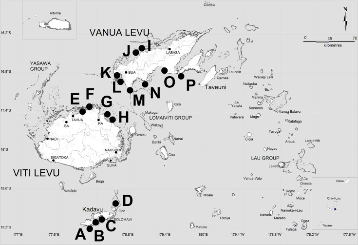
Fisheries and aquaculture industries worldwide remain reliant on seed supply from wild populations, with their success and sustainability dependent on consistent larval recruitment. Larval dispersal and recruitment in the marine environment are complex processes, influenced by a multitude of physical and biological factors. Biophysical modelling has increasingly been used to investigate dispersal and recruitment dynamics, for optimising management of fisheries and aquaculture resources. In the Fiji Islands, culture of the black-lip pearl oyster (Pinctada margaritifera) is almost exclusively reliant on wild-caught juvenile oysters (spat), through a national spat collection programme. This study used a simple Lagrangian particle dispersal model to investigate current-driven larval dispersal patterns, identify potential larval settlement areas and compare simulated with physical spat-fall, to inform targeted spat collection efforts. Simulations successfully identified country-wide patterns of potential larval dispersal and settlement from 2012-2015, with east-west variations between bi-annual spawning peaks and circulation associated with El Niño Southern Oscillation. Localised regions of larval aggregation were also identified and compared to physical spat-fall recorded at 28 spat collector deployment locations. Significant and positive correlations at these sites across three separate spawning seasons (r(26) = 0.435; r(26) = 0.438; r(26) = 0.428 respectively, p = 0.02), suggest high utility of the model despite its simplicity, for informing future spat collector deployment. Simulation results will further optimise black-lip pearl oyster spat collection activity in Fiji by informing targeted collector deployments, while the model provides a versatile and highly informative toolset for the fishery management and aquaculture of other marine taxa with similar life histories.


Conflict of interest statement

All authors read and approved the final manuscript, and declare that they have no competing interests.

Figures

Fig 1
Fig 1. Map of study area in the Fiji Islands adapted from Lal et al. [12].
Reef outlines are presented in dark grey. Site annotations depict spat collector deployment locations studied by Kishore et al. [22]. Collector deployment sites were as follows: Ravitaki (A), Galoa (B), Dravuwalu (C), Naqara (D), Vitawa (E), Malake A, B, C, D, E and F (F), Nacobau (G), Namarai A and B (H), Raviravi C (I), Raviravi A and B (J), Tavulomo A, B and C (K), Tavulomo D (L), Vuya (M), Navatu A and B (N), Urata (O) and Naweni A and B (P). The island of Rotuma and archipelago of Ono i Lau are shown inset.
Fig 2
Fig 2. Particle dispersal simulation results for 2012 and 2013 datasets (non-ENSO years).
Final (day 60) particle position plots are shown for spawning seasons 1 (A) and 2 (B) for 2012, and seasons 1 (C) and 2 (D) for 2013. All simulations were run for 60 days. Arrows denote the positions and trajectories of major particle flux patterns. Animations of these simulations are available as S1–S4 Gifs. Numbers denote the following localities: Viti Levu (1), Vanua Levu (2), Kadavu (3), Yasawa archipelago (4), Lau archipelago (5) and the Kingdom of Tonga (6).
Fig 3
Fig 3. Particle dispersal simulation results for 2014 and 2015 datasets (ENSO years).
Final (day 60) particle position plots are shown for spawning seasons 1 (A) and 2 (B) for 2014, and seasons 1 (C) and 2 (D) for 2015. All simulations were run for 60 days. Arrows denote the positions and trajectories of major particle flux patterns. Animations of these simulations are available as S5–S8 Gifs. Numbers denote the following localities: Viti Levu (1), Vanua Levu (2), Kadavu (3), Yasawa archipelago (4), Lau archipelago (5) and the Kingdom of Tonga (6).
Fig 4
Fig 4. Cumulative particle count heat maps for 2012 and 2013 datasets (non-ENSO years).
Final (day 60) particle counts are shown for spawning seasons 1 (A) and 2 (B) for 2012, and seasons 1 (C) and 2 (D) for 2013. Black circles denote the positions of spat collector deployments described by Kishore et al. [22]. The colour legend indicates the cumulative particle visit count within individual 10Km2 grid cells. Numbers denote the following localities: Viti Levu (1), Vanua Levu (2), Kadavu (3), Yasawa archipelago (4), Lau archipelago (5) and the Kingdom of Tonga (6).
Fig 5
Fig 5. Cumulative particle count heat maps for 2014 and 2015 datasets (ENSO years).
Final (day 60) particle counts are shown for spawning seasons 1 (A) and 2 (B) for 2014, and seasons 1 (C) and 2 (D) for 2015. Black circles denote the positions of spat collector deployments described by Kishore et al. [22]. The colour legend indicates the cumulative particle visit count within individual 10Km2 grid cells. Numbers denote the following localities: Viti Levu (1), Vanua Levu (2), Kadavu (3), Yasawa archipelago (4), Lau archipelago (5) and the Kingdom of Tonga (6).
Fig 6
Fig 6. Simulated cumulative 60-day particle counts for the 2013 second seasonal spawning peak period (November-December) at 28 spat collector deployment sites.
Spat collector sites are presented on the horizontal axis and the box and whisker plots for cumulative particle counts are displayed on the primary vertical (left) axis. Boxes indicate the limits of the first and third quartile values for cumulative particle counts at each collector deployment site, while upper and lower whiskers represent the maximum and minimum particle counts respectively. Physical counts of recruiting P. margaritifera spat are shown by the line plot in blue, and presented on the secondary vertical (right) axis for reference. Recruiting oyster counts are over a 10–15 month period from August 2013 to November 2014, and derived from Kishore et al. [22].
Fig 7
Fig 7. Simulated cumulative 60-day particle counts for the 2014 first seasonal spawning peak period (March-April) at 28 spat collector deployment sites.
Spat collector sites are presented on the horizontal axis and the box and whisker plots for cumulative particle counts are displayed on the primary vertical (left) axis. Boxes indicate the limits of the first and third quartile values for cumulative particle counts at each collector deployment site, while upper and lower whiskers represent the maximum and minimum particle counts respectively. Physical counts of recruiting P. margaritifera spat are shown by the line plot in blue, and presented on the secondary vertical (right) axis for reference. Recruiting oyster counts are over a 10–15 month period from August 2013 to November 2014, and derived from Kishore et al. [22].
Fig 8
Fig 8. Simulated cumulative 60-day particle counts for the 2014 second seasonal spawning peak period (November-December) at 28 spat collector deployment sites.
Spat collector sites are presented on the horizontal axis and the box and whisker plots for cumulative particle counts are displayed on the primary vertical (left) axis. Boxes indicate the limits of the first and third quartile values for cumulative particle counts at each collector deployment site, while upper and lower whiskers represent the maximum and minimum particle counts respectively. Physical counts of recruiting P. margaritifera spat are shown by the line plot in blue, and presented on the secondary vertical (right) axis for reference. Recruiting oyster counts are over a 10–15 month period from August 2013 to November 2014, and derived from Kishore et al. [22].
Fig 9
Fig 9. Pairwise matrix representation of modelled particle densities between 28 spat collector deployment sites during three spawning event simulations in 2013–2014.
Cell colours correspond to particle counts recorded between days 30 through 60 for each spawning simulation between collector deployment site pairs.

Similar articles

Cited by

References

    1. Hays GC (2017) Ocean currents and marine life. Current Biology 27: R470–R473. 10.1016/j.cub.2017.01.044 - DOI - PubMed
    1. Cowen RK, Sponaugle S (2009) Larval dispersal and marine population connectivity. Annual Review of Marine Science 1: 443–466. 10.1146/annurev.marine.010908.163757 - DOI - PubMed
    1. Nydam ML, Yanckello LM, Bialik SB, Giesbrecht KB, Nation GK, Peak JL (2017) Introgression in two species of broadcast spawning marine invertebrate. Biological Journal of the Linnean Society 120: 879–890.
    1. Pineda J, Reyns NB, Starczak VR (2009) Complexity and simplification in understanding recruitment in benthic populations. Population Ecology 51: 17–32.
    1. Gosling EM (2015) Fisheries and management of natural populations In: Gosling EM, editor. Marine Bivalve Molluscs. West Sussex, United Kingdom: Wiley Blackwell; pp. 270–324.

Publication types