Mapping Structural Connectivity Using Diffusion MRI: Challenges and Opportunities

Abstract

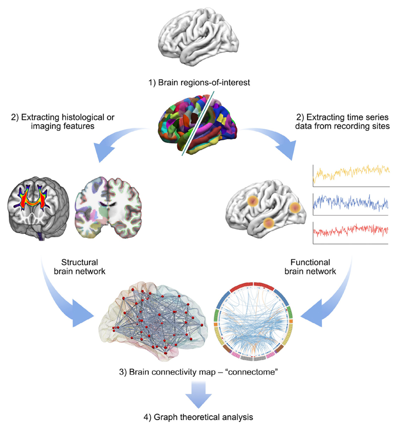
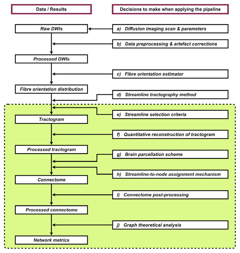
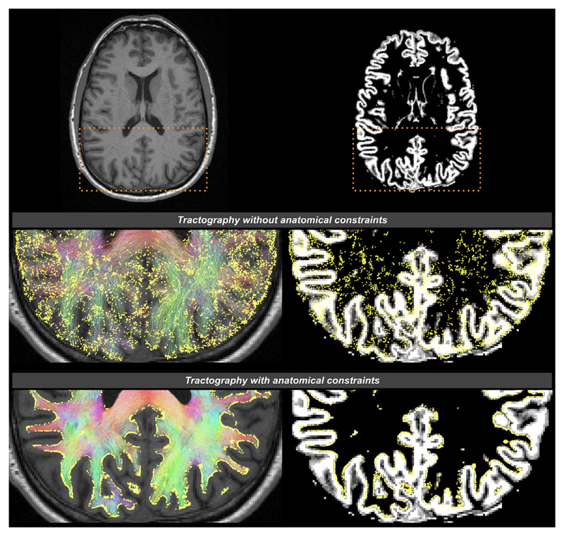
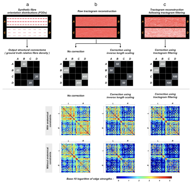
Diffusion MRI-based tractography is the most commonly-used technique when inferring the structural brain connectome, i.e., the comprehensive map of the connections in the brain. The utility of graph theory-a powerful mathematical approach for modeling complex network systems-for analyzing tractography-based connectomes brings important opportunities to interrogate connectome data, providing novel insights into the connectivity patterns and topological characteristics of brain structural networks. When applying this framework, however, there are challenges, particularly regarding methodological and biological plausibility. This article describes the challenges surrounding quantitative tractography and potential solutions. In addition, challenges related to the calculation of global network metrics based on graph theory are discussed.Evidence Level: 5Technical Efficacy: Stage 1.

Keywords: connectomics; diffusion MRI; graph theoretical analysis; network metrics; structural connectome; tractography.

Figure 1

A general overview of applying graph theoretical analysis to study structural (left branch) and functional (right branch) brain networks. A network or a graph is a collection of vertices (nodes) and their pairwise links (edges). A comprehensive set of all pairwise connections in the brain defines the topology of a brain network, providing a complete connectivity diagram of all associations among nodes and edges, i.e., a connectome. There are four essential components involved in this technique: 1) Defining nodes: Nodes are brain regions-of-interest; they are typically derived from an anatomical parcellation image data but can also be from more localized areas such as using electrodes, depending on the measurement technique. 2) Defining edges: Edges are the actual measure of relations between every node pair. They can be streamline connections from diffusion MRI tractography, inter-areal brain signal correlation/synchronization from resting-state functional connectivity, or other measures such as cortical thickness. 3) Constructing a network: This step integrates all the information from nodes and edges to generate a complete map of connectivity. The simplest representation of a network is using a 2D matrix (i.e., so-called connectivity matrix), but can also be visualized in various ways. 4) Graph theoretical analysis: In the present connectomics field, the most commonly-used method to calculate the characteristics of a network is by applying graph theory, which provides various global measures about the network topology.

Figure 2

An example processing workflow for generating an individual’s structural connectome using diffusion MRI data (an expanded version of the left branch in Fig. 1). Left column: Each box denotes the raw, interim, or final products of this pipeline. Right column: Each box describes the class of data processing involved in this pipeline. Within each procedure, there are many relevant options and parameters that have to be considered, where each choice can potentially affect the final output network metrics and the inference drawn from this technique. This shows the complexity of data processing in tractography-based structural connectomics research. The green box indicates the processing steps that are specifically discussed in the present article.

Figure 3

The effects of applying anatomical constraints on diffusion MRI streamlines tractography, shown on a transverse slice image of a human brain. The background images are a structural T1-weighted image on the left column, and the corresponding gray matter partial volume map following tissue segmentation on the right column. Streamlines are color-coded according to their orientations (red: left–right; green: anterior–posterior; blue: inferior–superior). The yellow spheres are the streamline endpoints. Top row: The dashed boxes indicate the zoomed brain areas shown in the middle and bottom rows. Middle row: Streamlines generated without anatomical priors; streamline endpoints distribute throughout the brain. Bottom row: Streamlines generated with anatomical priors; streamline endpoints only occur at the interface between GM and WM (demonstrated using Refs. 35, 42). It has been revealed that the considerable improvements in such streamline terminations provided by the use of anatomical constraints have significant influences on structural connectivity patterns and the outcomes of connectomic metrics.^,

Figure 4

The effects of quantitative tractogram postprocessing on subsequent quantification of connectome construction, illustrated using a synthetic example (upper panel) and human image data (bottom panel): Upper panel: (a) Fiber bundles A$B and C$D are simulated using synthetic fiber orientation distributions (FODs), where the size of FODs (i.e., apparent fiber density) in A$B is twice that in C$D. The relative fiber density of this synthetic FOD field is reflected in the connectome. (b) When running fiber-tracking, no matter whether seeding is performed uniformly from the whole (i.e., mimicking WM seeding) or from the extremities (i.e., mimicking seeding at the interface between GM and WM) of the fiber bundles, the same number of streamlines will be generated in both pathways. Obviously, the results do not comply with the synthetic ground-truth. The resultant connectome edges weighted by streamline density are therefore also biased in A$B and C$D when no correction is applied. Also, as inverse length scaling does not consider the size of FODs, it cannot correct for this type of quantification bias. (c) With the application of quantitative tractogram processing techniques (e.g., using Refs. 42, 45), the reconstructed streamline densities are rendered consistent with the underlying FOD field in A$B and C$D, making the connectome edges weighted by streamline density linearly proportional to the actual fiber density. Bottom panel: Group-averaged connectivity matrices generated from a cohort of healthy subjects. Probabilistic tractograms are generated with WM seeding; nodes are defined by the Desikan–Killiany atlas; edges are defined by streamline count. The first row shows the connectomes obtained from tractograms with anatomical constraints and then processed by different levels of quantitative bias correction (left: no correction; middle: correction using inverse length scaling; right: correction using tractogram filtering). For comparisons, the bottom row shows the results without anatomically-constrained tracking. L and R denote left and right hemispheres, respectively. The differences among these connectivity matrices are clearly visible, and indeed a range of popular connectomic metrics are significantly different. This figure is adapted from Ref. 43 with copyright permission.

Figure 5

Upper panel: An overview workflow of common approaches to prepare brain parcellation images in individual space. Following pre-processing of structural image data (usually T1-weighted images), individual’s brain parcellations can be obtained via: (a) applying brain cortical reconstruction and parcellation techniques (right branch), or (b) warping the brain atlas typically defined in standard space into individual space (left branch). The general procedure of the latter includes computing image transformations (denoted as T) by registering an individual’s anatomical images to those provided in the template space, and then pull the atlas from the template space to individual space via inverse transformation (denoted as T’). Bottom panel: Examples of brain parcellations transformed from a template/standard space into an individual’s space (left, e.g., automated anatomical labeling (AAL) atlas), or generated directly in the individual’s space via brain parcellation techniques (right, e.g., FreeSurfer parcellation; Desikan–Killiany atlas). Brain parcellations are overlaid on the structural T1-weighted images.

Figure 6

The effects of streamline-to-node assignment mechanisms on connectome construction, illustrated by a toy example (upper panel) and human image data (bottom panel): Upper panel: Examples of mechanisms used to assign streamlines to network nodes—streamlines shown in black; streamline endpoints denoted as E1 and E2; network nodes shown as colored voxels. The colored voxels added with red borders indicate the assigned nodes. As shown in this figure, even for an identical streamline, the assigned nodes (and therefore the outcome connectivity) among those streamline-to-node assignment methods are all different, suggesting that the design of such a mechanism can have direct influence on connectome quantification (see Ref. 44 for detailed explanations). Bottom panel: Group-averaged connectivity matrices generated from a cohort of healthy subjects. Probabilistic tractograms are generated; nodes are defined by Desikan–Killiany atlas; edges are defined by weighted streamline counts as provided by quantitative tractogram processing. In the upper row, the matrices are obtained using tractography with anatomical constraints, where the three streamline-to-node assignment mechanisms shown in the upper panel are used for connectome construction. For comparisons, the bottom row shows the results without anatomically-constrained tracking. L and R denote left and right hemispheres, respectively. The outcome connectivity pattern and connectomic metrics are significantly different among these connectivity matrices, highlighting the necessity of selecting an appropriate strategy for connectome construction. This figure is adapted from Ref. 44 with copyright permission.

Figure 7

The effects of the misalignment between image-intensity-based tissue segmentation and brain parcellation on the assignment of streamlines to network nodes: Upper panel: (a) With the application of anatomical constraints (e.g., Ref. 35), streamline endpoints (colored in purple) occur at the GM–WM interface or within the subcortical GM. (b) Due to factors such as discretization of structural labels, many of these endpoints (purple points) do not locate inside the, for example, FreeSurfer parcellation image (blue ribbon) and thus are not assigned to a label. (c) The T1 image shown in (a,b) is replaced by the GM partial volume maps derived from intensity-based tissue segmentation. (d) A zoom region of (c) illustrates the discrepancy (pointed by arrows) between tissue segmentation and brain parcellation, revealing that streamlines cannot be assigned purely based on the voxels where the endpoints reside. Bottom panel: The discrepancies also present in subcortical GM, and in fact could be even crucial when parcellation images are prepared by transforming an atlas to an individual’s space (i.e., the left branch of Fig. 5). This is because the degree of misalignment between subcortical GM segmentations and brain parcellations could be increased by the registration error. As an example: (e) The AAL atlas is coregistered to individuals’ data via linear and nonlinear transformations. The background shows a T1-weighted image slice of the subject. (f) The background image is replaced by the GM partial volume map obtained from tissue segmentation. (g) The red arrows point to the considerable misalignment between two images at the thalami regions.

References

1. Bullmore E, Sporns O. Complex brain networks: Graph theoretical analysis of structural and functional systems. Nat Rev Neurosci. 2009;10:186–198. - PubMed
1. Hagmann P, Cammoun L, Gigandet X, et al. Mapping the structural core of human cerebral cortex. PLoS Biol. 2008;6:e159. - PMC - PubMed
1. Sporns O, Tononi G, Kötter R. The human connectome: A structural description of the human brain. PLoS Comp Biol. 2005;1:e42. - PMC - PubMed
1. Sporns O. The human connectome: A complex network. Ann N Y Acad Sci. 2011;1224:109–125. - PubMed
1. Bassett DS, Bullmore E. Small-world brain networks. Neuroscientist. 2006;12:512–523. - PubMed
Publication types