Shape morphology of dipolar domains in planar and spherical monolayers

Abstract

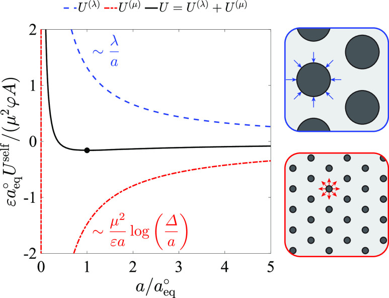
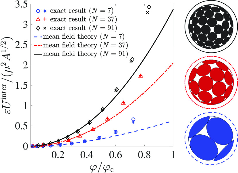
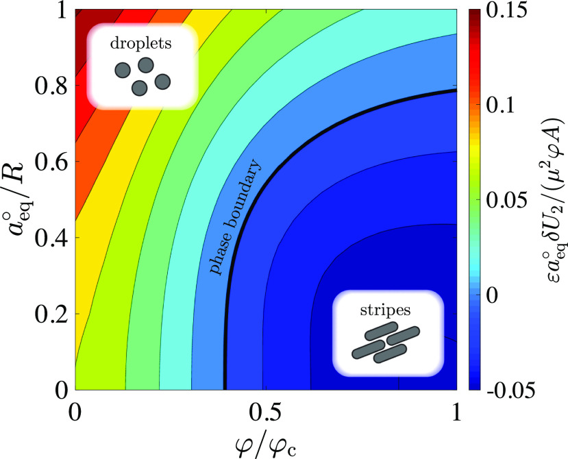
We present a continuum theory for predicting the equilibrium shape and size of dipolar domains formed during liquid-liquid phase coexistence in planar and spherical monolayers. Our main objective is to assess the impact of the monolayer surface curvature on domain morphology. Following previous investigators, we base our analysis around minimizing the free energy, with contributions from line tension and electrostatic dipolar repulsions. Assuming a monodisperse system of circularly symmetric domains, we calculate self-energies and interaction energies for planar and spherical monolayers and determine the equilibrium domain size from the energy minima. We subsequently evaluate the stability of the circularly symmetric domain shapes to an arbitrary, circumferential distortion of the perimeter via a linear stability analysis. We find that the surface curvature generally promotes the formation of smaller, circularly symmetric domains instead of larger, elongated domains. We rationalize these results by examining the effect of the curvature on the intra- and inter-domain dipolar repulsions. We then present a phase diagram of domain shape morphologies, parameterized in terms of the domain area fraction and the monolayer curvature. For typical domain dimensions of 1-30 µm, our theoretical results are relevant to monolayers (and possibly also bilayers) in liquid-liquid phase coexistence with radii of curvature of 1-100 µm.

FIG. 1.

Dipolar domains in (a) planar and (b) spherical monolayers.

FIG. 2.

Isolated circular disk of radius a in the xy plane with dipole moment density $\mathit{\mu }=\mu \widehat{\mathbf{z}}$ and line tension λ.

FIG. 3.

The two contributions to the planar self-energy U^self as a function of the disk radius a [cf. Eq. (19)]. The black dot indicates the energy minimum at the (dilute) equilibrium radius $a=a_{\mathrm{e}\mathrm{q}}^{◦}$. The forces associated with line tension and dipolar repulsions are depicted pictorially on the right. The parameters used for the plots are ελ/μ² = 0.66 and Δ = 5 Å.

FIG. 4.

Two co-planar circular disks of radius a whose centers are separated by a distance b at an angle ω relative to the x-axis.

FIG. 5.

The planar pairwise interaction energy $U_{12}^{\left(\mu \right)}$ as a function of the ratio of the separation distance b to the disk radius a. Shown are the exact result (22) as well as the two asymptotic limits (23) and (24).

FIG. 6.

The planar interaction energy U^inter plotted against the relative area fraction φ/φ_c, where φ = Nπa²/A and φ_c ≈ 0.907 is given by Eq. (29). McConnell’s result (thin curves) is given by Eq. (26). The mean field approximation (thick curves) is given by Eq. (28). The exact result (markers) is found by summing the exact pairwise interaction energy (22) over a hexagonal lattice of N circular disks, shown pictorially on the right in the close-packing limit φ = φ_c.

FIG. 7.

The nth planar energy perturbation δU_n plotted against the disk radius a for the first few mode numbers n = 2, 3, 4, 5. The neutral stability boundary a = a_n at δU_n = 0 is marked with an open circle for each mode. A pictorial representation of each n-fold shape distortion is shown on the right. The parameters used for the plots are ελ/μ² = 0.66 and Δ = 5 Å.

FIG. 8.

Isolated spherical cap at r = R with cap angle α, dipole moment density $\mathit{\mu }=\mu \widehat{\mathbf{r}}$, and line tension λ.

FIG. 9.

The spherical self-energy U^self plotted against the arc length Rα for various dimensionless curvatures $a_{\mathrm{e}\mathrm{q}}^{◦}/R$ [cf. Eq. (45)]. The planar limit ($a_{\mathrm{e}\mathrm{q}}^{◦}/R=0$) is given by Eq. (19) with a = Rα. The hemispherical limit corresponds to the energy for which α = π/2. For each curve, the black dot indicates the energy minimum at the equilibrium arc length $R{\alpha }_{\mathrm{e}\mathrm{q}}^{◦}$. (Inset) The equilibrium arc length $R{\alpha }_{\mathrm{e}\mathrm{q}}^{◦}$ plotted against the dimensionless curvature $a_{\mathrm{e}\mathrm{q}}^{◦}/R$, as given by the solution of Eq. (46). The parameters used for the plots are ελ/μ² = 0.66 and Δ = 5 Å.

FIG. 10.

The critical area fraction φ_c,N plotted against the number of domains N for a lattice of caps on a sphere. The thick, solid curves were generated using lattice points taken from electronic databases. Globally optimized results for the Thomson lattice of point charges up to N = 400 were tabulated by Wales and Ulker (green solid curve). The Tammes lattice points up to N = 130 were tabulated by Hardin, Sloane, and Smith (black solid curve). The thin, dotted curves indicate our own, locally optimized calculations of the lattice points for the generalized Thomson problem, both for point charges (blue dotted curve) and point dipoles (red dotted curve). The planar close-packing limit for a hexagonal lattice φ_c ≈ 0.907 is given by Eq. (29).

FIG. 11.

Two spherical caps at r = R of angle α, whose centers are separated by the polar angle β and azimuthal angle ω.

FIG. 12.

The spherical pairwise interaction energy $U_{12}^{\left(\mu \right)}$ as a function of the separation angle β for various cap angles α. Shown are the exact result (50) (markers) as well as the far-field (dipole–dipole) approximation (51) (curves).

FIG. 13.

(a) Two vertically oriented point dipoles separated by a distance Rβ in a horizontal plane. (b) Two radially oriented point dipoles separated by an angle β on a sphere of radius R is equivalent to two non-parallel dipoles separated by a distance 2R sin(β/2) < Rβ in a plane. The oblique alignment and shorter separation distance result in a stronger repulsion between the dipoles.

FIG. 14.

The spherical interaction energy U^inter plotted against the relative area fraction φ/φ_c, where φ = N(1 − cos α)/2 and φ_c ≈ 0.907 is given by Eq. (29). The mean field approximation (curves) is given by Eq. (54). The exact result is found by summing the exact pairwise interaction energy (50) over an array of N spherical caps arranged in a Thomson dipole lattice (open-face markers) or a Tammes lattice (symbols). The Tammes lattice points were obtained from Hardin, Sloane, and Smith and are shown pictorially on the right for the close-packing limit φ = φ_c,N < φ_c.

FIG. 15.

(a) The equilibrium arc length Rα_eq plotted against the relative area fraction φ/φ_c for various dimensionless curvatures $a_{\mathrm{e}\mathrm{q}}^{◦}/R$. Here, φ = N(1 − cos α)/2 and φ_c ≈ 0.907 is given by Eq. (29). Each curve is obtained by solving the transcendental Eq. (56) numerically for particular values of φ and $a_{\mathrm{e}\mathrm{q}}^{◦}/R$. The planar limit Rα_eq = a_eq is given by Eq. (32). (b) The equilibrium number density N_eq/A predicted by Eqs. (56) and (59). The restrictions of the theory produce a continuous, rather than discrete, two-parameter family of solutions for N_eq as a function of $a_{\mathrm{e}\mathrm{q}}^{◦}/R$ and φ.

FIG. 16.

The second spherical energy perturbation δU₂ plotted against the arc length Rα for various dimensionless curvatures $a_{\mathrm{e}\mathrm{q}}^{◦}/R$. The neutral stability boundary α = α₂ at δU₂ = 0 is marked with an open circle for each curve. (Inset) The critical arc length $R{\alpha }_2^{◦}$ plotted against the curvature 1/R, as given by the solution of Eq. (67). For dimensionless curvatures $a_{\mathrm{e}\mathrm{q}}^{◦}/R>0.8$, no solution of Eq. (67) is found and the circularly symmetric shape is always stable. The parameters used for the plots are ελ/μ² = 0.66 and Δ = 5 Å.

FIG. 17.

Phase diagram of domain shapes. Isocontours of the energy perturbation δU₂ are plotted at the equilibrium cap angle α = α_eq as a function of the dimensionless curvature $a_{\mathrm{e}\mathrm{q}}^{◦}/R$ and relative area fraction φ/φ_c. The phase boundary between the droplet and stripe phases is demarcated by the solid line and corresponds to the neutral stability boundary δU₂ = 0, where α_eq = α₂. The parameters used for the plots are ελ/μ² = 0.66 and Δ = 5 Å.

FIG. 18.

The potential and field lines for a polarized circular disk.

FIG. 19.

The potential and field lines for a polarized spherical cap.

References

1. Israelachvili J. N., Intermolecular and Surface Forces, 3rd ed. (Elsevier, 2011).
1. Braun R. J., “Dynamics of the tear film,” Annu. Rev. Fluid Mech. 44, 267–297 (2012).10.1146/annurev-fluid-120710-101042 - DOI
1. Zasadzinski J. A., Ding J., Warriner H. E., Bringezu F., and Waring A. J., “The physics and physiology of lung surfactants,” Curr. Opin. Colloid Interface Sci. 6, 506–513 (2001).10.1016/s1359-0294(01)00124-8 - DOI
1. Moy V. T., Keller D. J., and McConnell H. M., “Molecular order in finite two-dimensional crystals of lipid at the air-water interface,” J. Phys. Chem. 92, 5233–5238 (1988).10.1021/j100329a033 - DOI
1. Dufrêne Y. F., Barger W. R., Green J.-B. D., and Lee G. U., “Nanometer-scale surface properties of mixed phospholipid monolayers and bilayers,” Langmuir 13, 4779–4784 (1997).10.1021/la970221r - DOI