A community-maintained standard library of population genetic models

Abstract

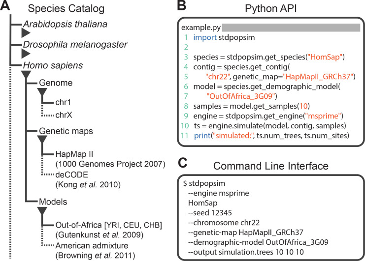
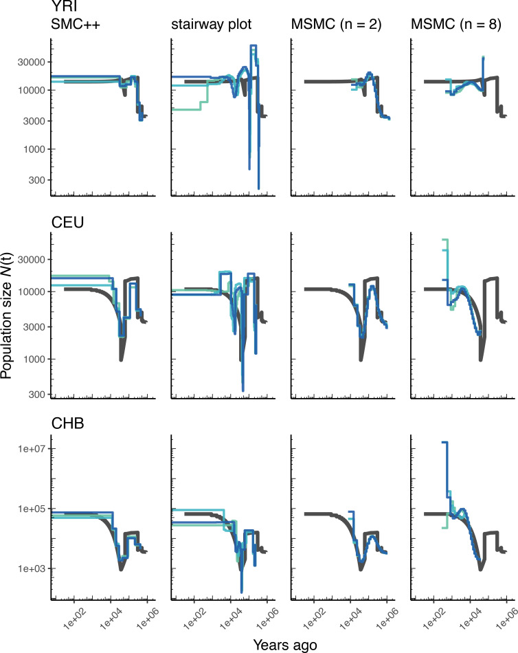
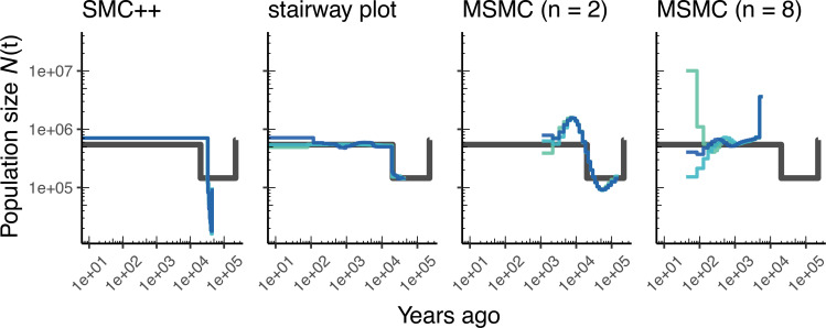
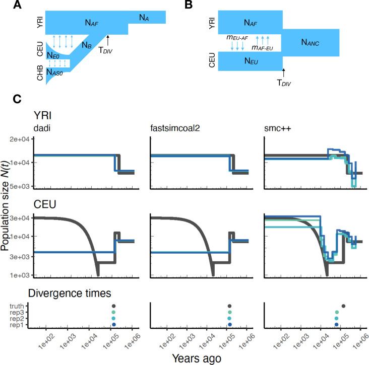
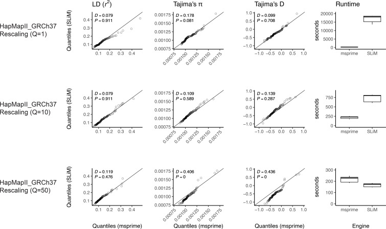
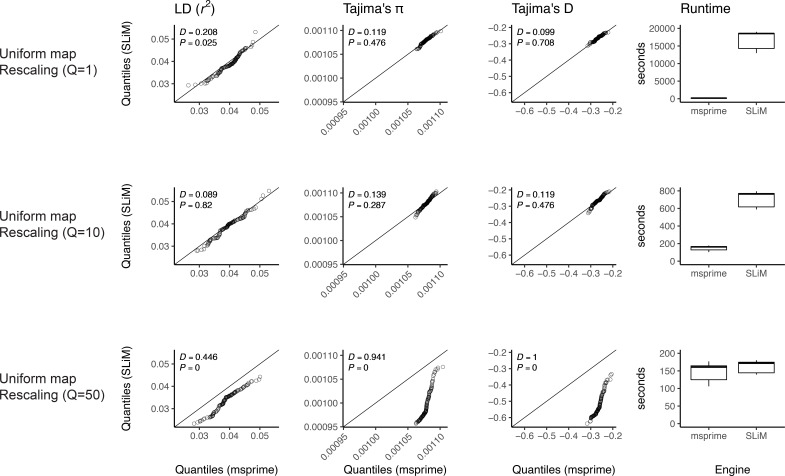
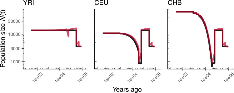
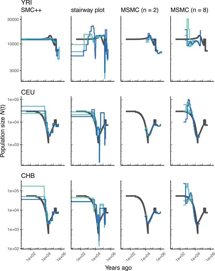
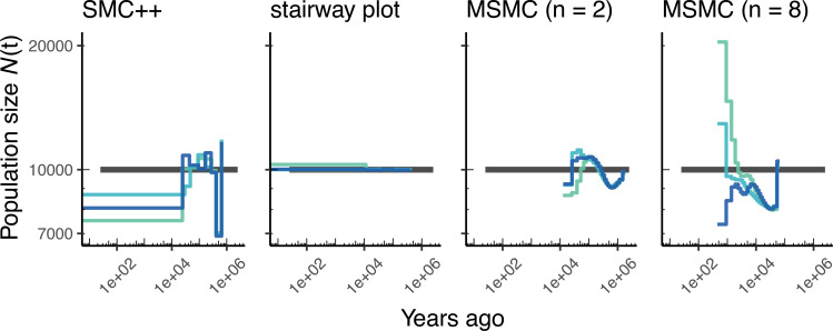
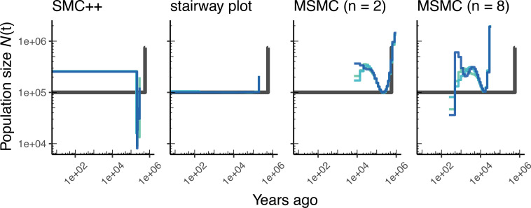
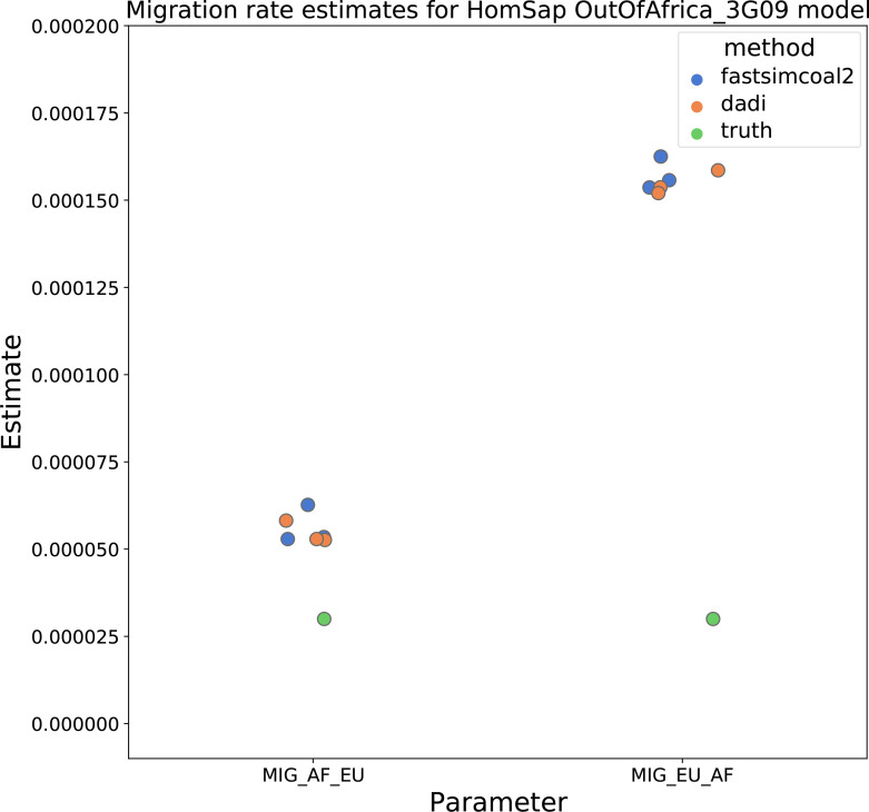
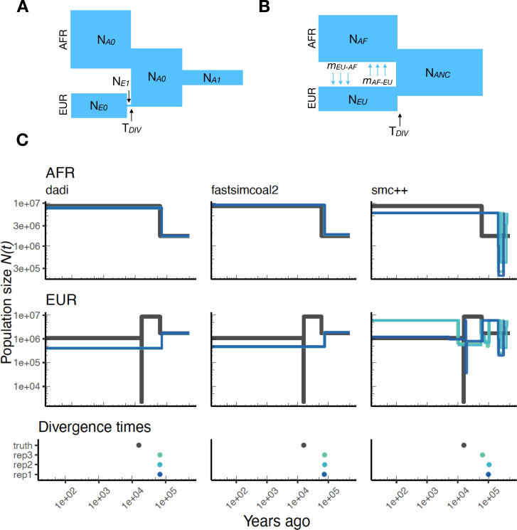
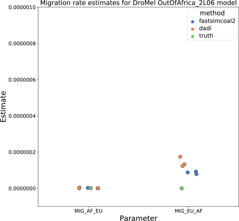
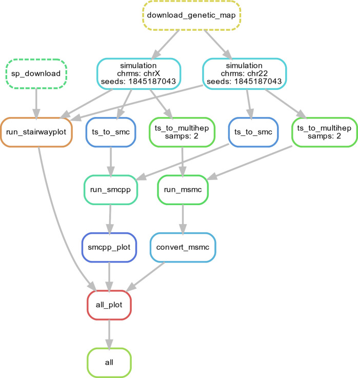
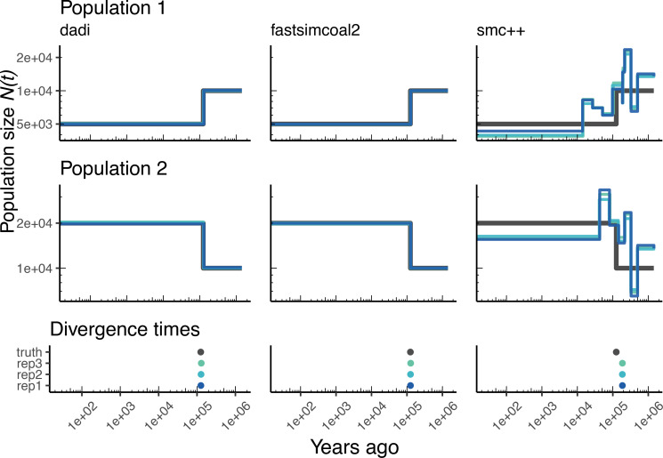
The explosion in population genomic data demands ever more complex modes of analysis, and increasingly, these analyses depend on sophisticated simulations. Recent advances in population genetic simulation have made it possible to simulate large and complex models, but specifying such models for a particular simulation engine remains a difficult and error-prone task. Computational genetics researchers currently re-implement simulation models independently, leading to inconsistency and duplication of effort. This situation presents a major barrier to empirical researchers seeking to use simulations for power analyses of upcoming studies or sanity checks on existing genomic data. Population genetics, as a field, also lacks standard benchmarks by which new tools for inference might be measured. Here, we describe a new resource, stdpopsim, that attempts to rectify this situation. Stdpopsim is a community-driven open source project, which provides easy access to a growing catalog of published simulation models from a range of organisms and supports multiple simulation engine backends. This resource is available as a well-documented python library with a simple command-line interface. We share some examples demonstrating how stdpopsim can be used to systematically compare demographic inference methods, and we encourage a broader community of developers to contribute to this growing resource.

Keywords: computational biology; evolutionary biology; human; open source; reproducibility; simulation; systems biology.

Figure 1.. Structure of stdpopsim.

(A) The hierarchical organization of the stdpopsim catalog contains all model simulation information within individual species (expanded information shown here for H. sapiens only). Each species is associated with a representation of the physical genome, and one or more genetic maps and demographic models. Dotted lines indicate that only a subset of these categories is shown. At right we show example code to specify and simulate models using (B) the python API or (C) the command line interface.

Figure 2.. Comparing estimates of N⁢(t) in humans.

Here we show estimates of population size over time ($N(t)$) inferred using four different methods: smc++, stairway plot, and MSMC with $n=2$ and $n=8$ samples. Data were generated by simulating replicate human genomes under the OutOfAfricaArchaicAdmixture_5R19 model (Ragsdale and Gravel, 2019) and using the HapMapII_GRCh37 genetic map (Frazer et al., 2007). From top to bottom, we show estimates for each of the three populations in the model (YRI, CEU, and CHB). In shades of blue we show the estimated $N(t)$ trajectories for each of three replicates. As a proxy for the ‘truth’, in black we show inverse coalescence rates as calculated from the demographic model used for simulation (see text).

Figure 3.. Comparing estimates of N⁢(t) in Drosophila.

Population size over time ($N(t)$) estimated from an African population sample. Data were generated by simulating replicate D. melanogaster genomes under the African3Epoch_1S16 model (Sheehan and Song, 2016) with the genetic map of Comeron et al., 2012. In shades of blue we show the estimated $N(t)$ trajectories for each replicate. As a proxy for the ‘truth’, in black we show inverse coalescence rates as calculated from the demographic model used for simulation (see text).

Figure 4.. Parameters estimated using a multi-population human model.

Here we show estimates of $N(t)$ inferred using $\partial a\partial i$, fastsimcoal2, and smc++. (A) Data were generated by simulating replicate human genomes under the OutOfAfrica_3G09 model and using the HapMapII_GRCh37 genetic map inferred in Frazer et al., 2007. (B) For $\partial a\partial i$ and fastsimcoal2 we show parameters inferred by fitting the depicted IM model, which includes population sizes, migration rates, and a split time between CEU and YRI samples. (C) Population size estimates for each population (rows) from $\partial a\partial i$, fastsimcoal2, and smc++ (columns). In shades of blue we show $N(t)$ trajectories estimated from each simulation, and in black simulated population sizes for the respective population. The population split time, $T_{DIV}$, is shown at the bottom (simulated value in black and inferred values in blue), with a common $x$-axis to the population size panels.

Appendix 1—figure 1.. Validating the SLiM engine backend under a genetic map.

Here, we validate our integration of the SLiM (Haller et al., 2019; Haller and Messer, 2019) engine backend. We show quantile-quantile plots between SLiM and msprime engines for three population genetic summary statistics: r², Tajima’s $\pi$, and Tajima’s D. Additionally, we show runtimes for generating each simulation replicate. Data were generated by simulating 100 replicates of human chromosome 22 under the AncientEurasia_9K19 model (Kamm et al., 2019) using the HapMapII_GRCh37 genetic map (Frazer et al., 2007). 12 samples were drawn from each population (excluding basal Eurasians). From top to bottom, we show results using three scaling factors for the population sizes: Q = 1, Q = 10, and Q = 50. Kolmogorov-Smirnov two-sample test statistics (D) and p-values are shown, testing the null hypothesis that the quantiles were drawn from the same continuous distribution.

Appendix 1—figure 2.. Validating the SLiM engine backend under uniform recombination.

Here, we validate our integration of the SLiM (Haller et al., 2019; Haller and Messer, 2019) engine backend. We show quantile-quantile plots between SLiM and msprime engines for three population genetic summary statistics: r², Tajima’s $\pi$, and Tajima’s D. Additionally, we show runtimes for generating each simulation replicate. Data were generated by simulating 100 replicates of human chromosome 22 under the AncientEurasia_9K19 model (Kamm et al., 2019) using a uniform rate of recombination across the chromosome. 12 samples were drawn from each population (excluding basal Eurasians). From top to bottom, we show results using three scaling factors for the population sizes: Q = 1, Q = 10, and Q = 50. Kolmogorov-Smirnov two-sample test statistics (D) and p-values are shown, testing the null hypothesis that the quantiles were drawn from the same continuous distribution.

Appendix 1—figure 3.. Comparing simulated population sizes and inverse coalescence rates in humans.

Data are shown from human genomes under the OutOfAfricaArchaicAdmixture_5R19 model (Ragsdale and Gravel, 2019) and using the HapMapII_GRCh37 genetic map (Frazer et al., 2007). From left to right, we show sizes for each of the three populations in the model: YRI, CEU, and CHB. We plot the simulated sizes for each population in black, and in red we plot inverse coalescence rates as calculated from the demographic model used for simulation (see text). In this specific model, these two measures are near identical, but in other models with higher migration rates we expect to see a larger departure between the two.

Appendix 1—figure 4.. Comparing estimates of N⁢(t) in humans.

Estimates of population size over time ($N(t)$) inferred using four different methods, smc++, stairway plot, and MSMC with $n=2$ and $n=8$. Data were generated by simulating replicate human genomes under the OutOfAfrica_3G09 model (Gutenkunst et al., 2009) and using the HapMapII_GRCh37 genetic map (Frazer et al., 2007). From top to bottom, we show estimates for each of the three populations in the model: YRI, CEU, and CHB. In shades of blue, we show the estimated $N(t)$ trajectories for each replicate. As a proxy for the ‘truth’, in black we show inverse coalescence rates as calculated from the demographic model used for simulation (see text).

Appendix 1—figure 5.. Comparing estimates of N⁢(t) in humans.

Here, we show estimates of population size over time ($N(t)$) inferred using fourdifferent methods, smc+, and stairway plot, and MSMC with $n=2$ and $n=8$. Data were generated by simulating replicate human genomes under a constant sized population model with $N={10}^4$ and using the HapMapII_GRCh37 genetic map (Frazer et al., 2007). As a proxy for the ‘truth’, in black we show inverse coalescence rates as calculated from the demographic model used for simulation (see text).

Appendix 1—figure 6.. Comparing estimates of N⁢(t) in A. thaliana.

Here, we show estimates of population size over time ($N(t)$) inferred using four different methods, smc++, and stairway plot, and MSMC with $n=2$ and $n=8$. Data were generated by simulating replicate A. thaliana genomes under the African2Epoch_1H18 model (Durvasula et al., 2017) and using the SalomeAveraged_TAIR7 genetic map (Salomé et al., 2012). As a proxy for the ‘truth’, in black we show inverse coalescence rates as calculated from the demographic model used for simulation (see text).

Appendix 1—figure 7.. Migration rate estimates for the human Gutenkunst model.

Here, we show inferred migration rates from $\partial a\partial i$ and fastsimcoal2. Data were generated by simulating replicate human genomes under the Gutenkunst et al., 2009 model and using the genetic map inferred in Frazer et al., 2007. Directional migration from Europe to Africa is represented as $MIG\mathrm{\_}AF\mathrm{\_}EU$ and migration from Africa to Europe is represented as $MIG\mathrm{\_}EU\mathrm{\_}AF$. Note that the $x$-axis coordinates are arbitrary.

Appendix 1—figure 8.. Parameters estimated using a two-population Drosophila model.

Here, we show estimates of $N(t)$ inferred using $\partial a\partial i$, fastsimcoal2, and smc++. Data were generated by simulating replicate Drosophila genomes under the Li and Stephan, 2006 model and using the genetic map inferred in Comeron et al., 2012. See legend of Figure 4 for details. In shades of blue, we show the estimated $N(t)$ trajectories for each replicate. In black we show the simulated population sizes.

Appendix 1—figure 9.. Migration rate parameters estimated under a two-population Drosophila model.

Here, we show inferred migration rates from $\partial a\partial i$ and fastsimcoal2. Data were generated by simulating replicate Drosophila genomes under the Li and Stephan, 2006 model and using the genetic map inferred in Comeron et al., 2012. Directional migration from Europe to Africa is represented as $MIG\mathrm{\_}AF\mathrm{\_}EU$ and migration from Africa to Europe is represented as $MIG\mathrm{\_}EU\mathrm{\_}AF$. Note that the $x$-axis coordinates are arbitrary.

Appendix 1—figure 10.. Workflow for our N(t) inference methods comparison.

Here, we show single replicate for two chromosomes, chr22 and chrX, simulated under the HomSap OutOfAfrica_3G09 demographic model, with a HapmapII_GRCh37 genetic map. Note that the data used as input by all inference methods smc++, MSMC, and stairway plot, come from the same set of simulations.

Appendix 1—figure 11.. Parameters estimated from a generic IM model Here we show estimates of N⁢(t) inferred using ∂⁡a⁢∂⁡i, fastsimcoal2, and smc++.

Data were generated by simulating under a generic IM model with a human genome and Frazer et al., 2007 genetic map. In shades of blue we show the estimated $N(t)$ trajectories for each replicate. In black we show the simulated population sizes.

References

1. Adrion JR, Galloway JG, Kern AD. Predicting the landscape of recombination using deep learning. Molecular Biology and Evolution. 2020;37:1790–1808. doi: 10.1093/molbev/msaa038. - DOI - PMC - PubMed
1. Alachiotis N, Stamatakis A, Pavlidis P. OmegaPlus: a scalable tool for rapid detection of selective sweeps in whole-genome datasets. Bioinformatics. 2012;28:2274–2275. doi: 10.1093/bioinformatics/bts419. - DOI - PubMed
1. Andrews KR, Good JM, Miller MR, Luikart G, Hohenlohe PA. Harnessing the power of RADseq for ecological and evolutionary genomics. Nature Reviews Genetics. 2016;17:81–92. doi: 10.1038/nrg.2015.28. - DOI - PMC - PubMed
1. Beichman AC, Phung TN, Lohmueller KE. Comparison of single genome and allele frequency data reveals discordant demographic histories. G3: Genes, Genomes, Genetics. 2017;7:3605–3620. doi: 10.1534/g3.117.300259. - DOI - PMC - PubMed
1. Beichman AC, Huerta-Sanchez E, Lohmueller KE. Using genomic data to infer historic population dynamics of nonmodel organisms. Annual Review of Ecology, Evolution, and Systematics. 2018;49:433–456. doi: 10.1146/annurev-ecolsys-110617-062431. - DOI
Publication types
LinkOut - more resources