A Simulation of a COVID-19 Epidemic Based on a Deterministic SEIR Model

Abstract

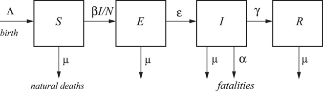
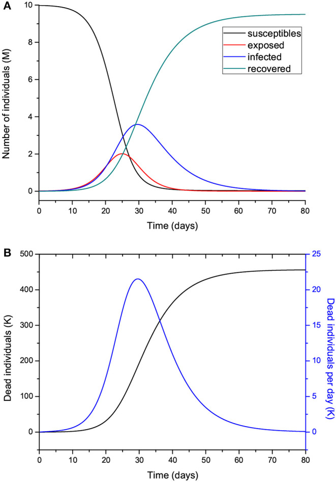
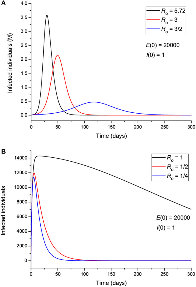
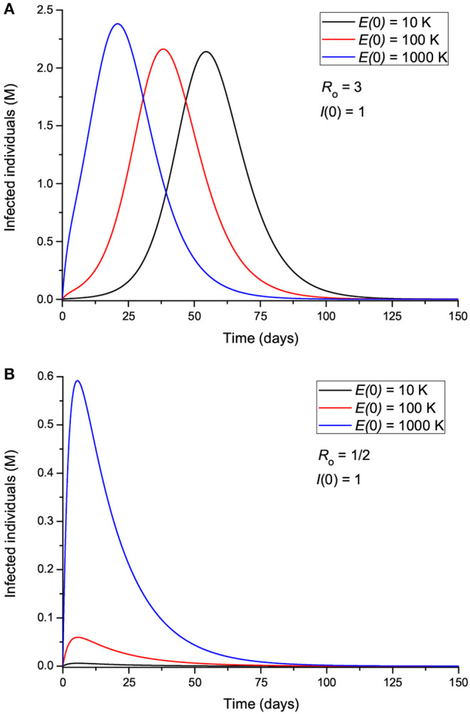
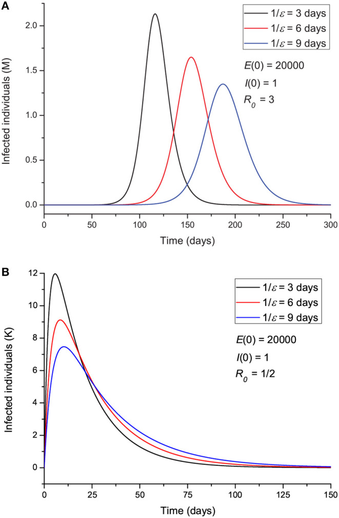
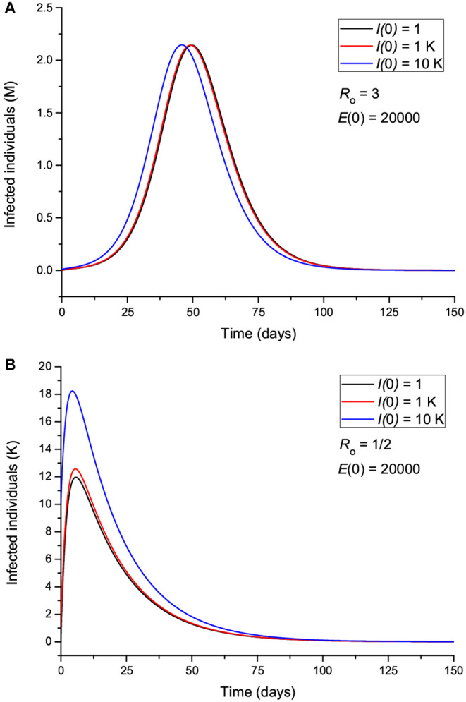
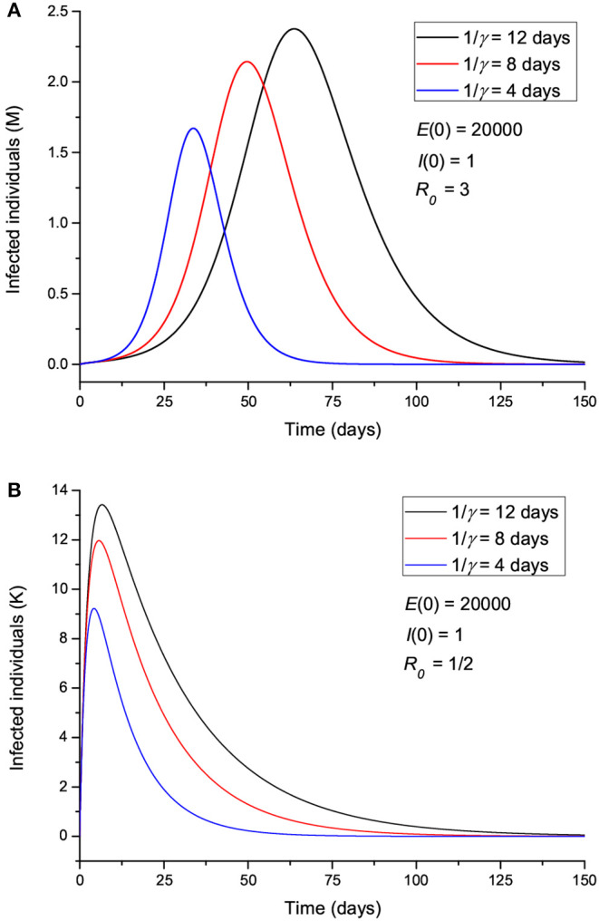
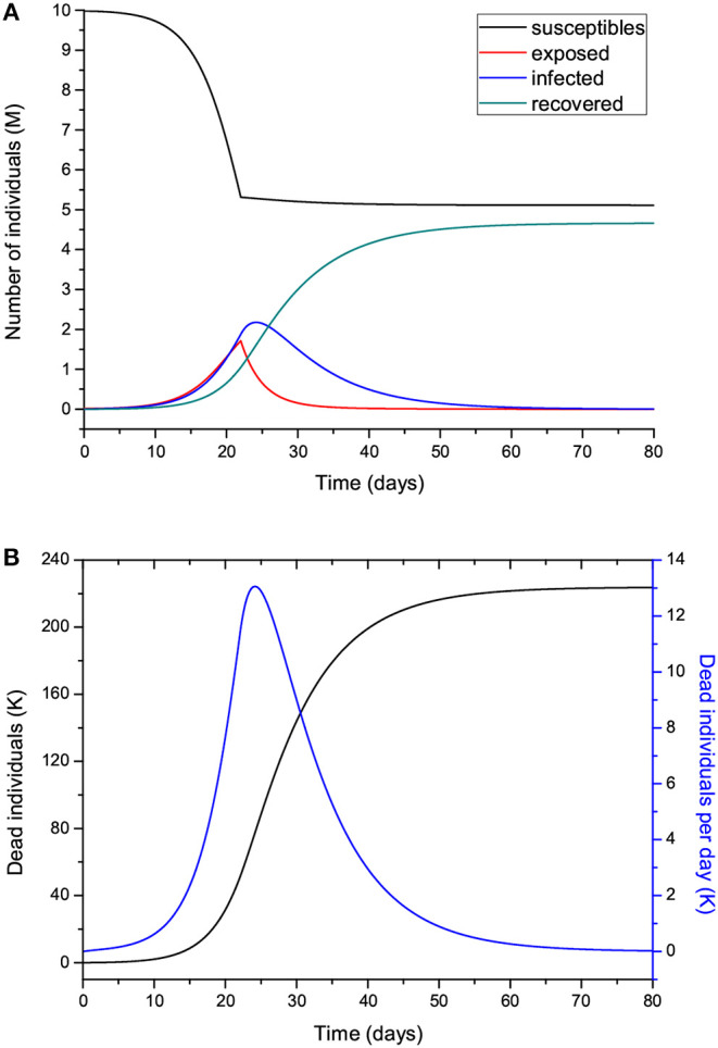
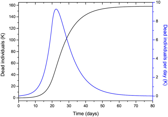
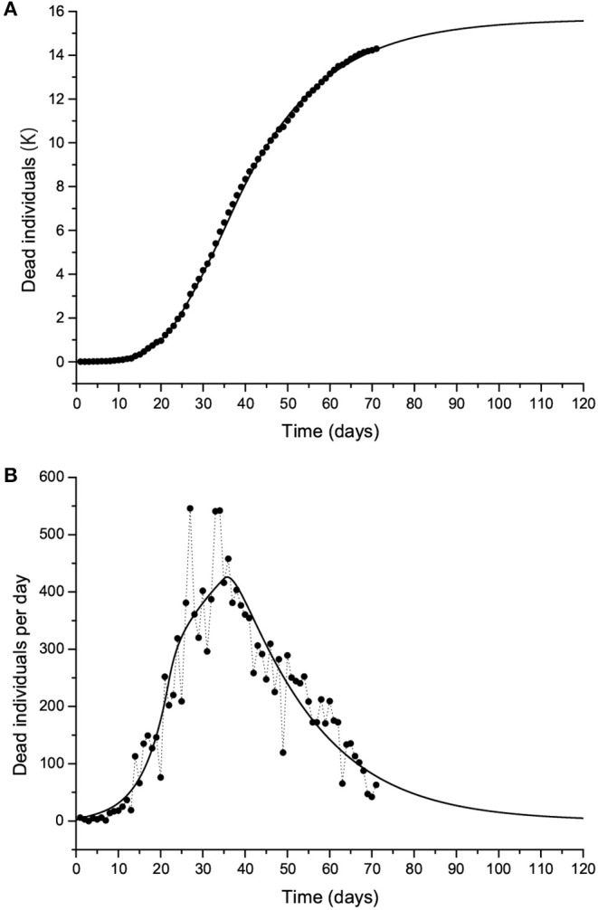
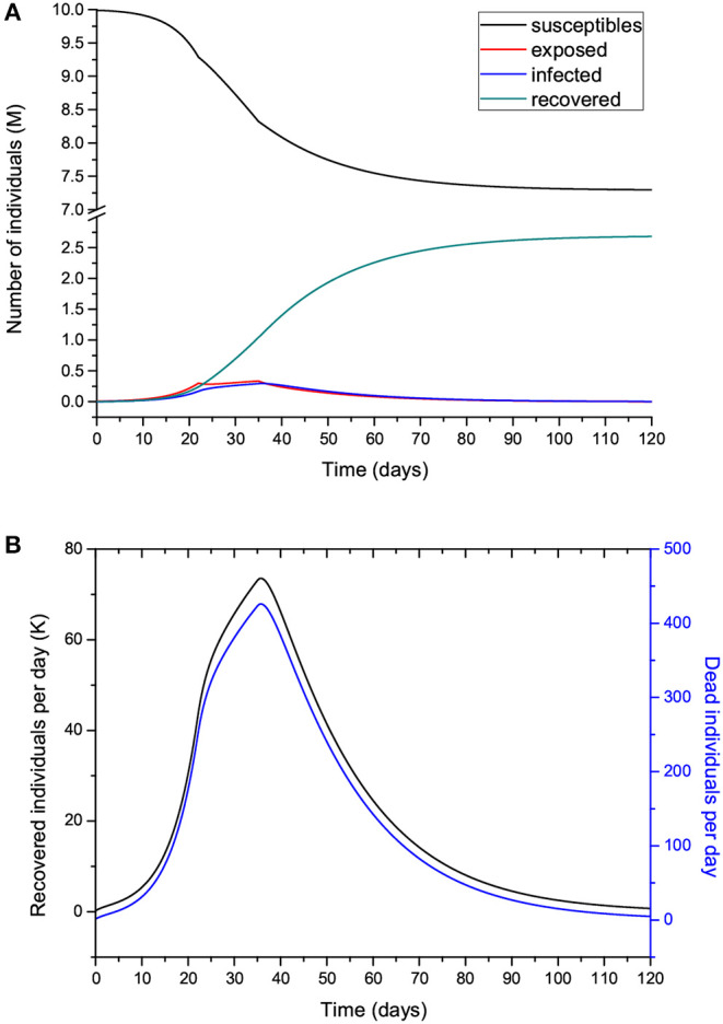
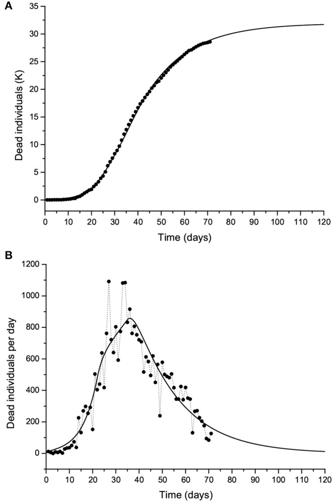
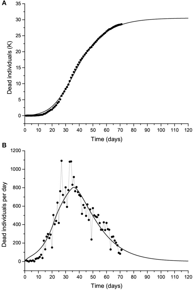
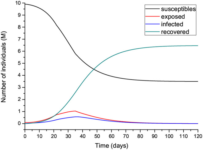
An epidemic disease caused by a new coronavirus has spread in Northern Italy with a strong contagion rate. We implement an SEIR model to compute the infected population and the number of casualties of this epidemic. The example may ideally regard the situation in the Italian Region of Lombardy, where the epidemic started on February 24, but by no means attempts to perform a rigorous case study in view of the lack of suitable data and the uncertainty of the different parameters, namely, the variation of the degree of home isolation and social distancing as a function of time, the initial number of exposed individuals and infected people, the incubation and infectious periods, and the fatality rate. First, we perform an analysis of the results of the model by varying the parameters and initial conditions (in order for the epidemic to start, there should be at least one exposed or one infectious human). Then, we consider the Lombardy case and calibrate the model with the number of dead individuals to date (May 5, 2020) and constrain the parameters on the basis of values reported in the literature. The peak occurs at day 37 (March 31) approximately, with a reproduction ratio R₀ of 3 initially, 1.36 at day 22, and 0.8 after day 35, indicating different degrees of lockdown. The predicted death toll is approximately 15,600 casualties, with 2.7 million infected individuals at the end of the epidemic. The incubation period providing a better fit to the dead individuals is 4.25 days, and the infectious period is 4 days, with a fatality rate of 0.00144/day [values based on the reported (official) number of casualties]. The infection fatality rate (IFR) is 0.57%, and it is 2.37% if twice the reported number of casualties is assumed. However, these rates depend on the initial number of exposed individuals. If approximately nine times more individuals are exposed, there are three times more infected people at the end of the epidemic and IFR = 0.47%. If we relax these constraints and use a wider range of lower and upper bounds for the incubation and infectious periods, we observe that a higher incubation period (13 vs. 4.25 days) gives the same IFR (0.6 vs. 0.57%), but nine times more exposed individuals in the first case. Other choices of the set of parameters also provide a good fit to the data, but some of the results may not be realistic. Therefore, an accurate determination of the fatality rate and characteristics of the epidemic is subject to knowledge of the precise bounds of the parameters. Besides the specific example, the analysis proposed in this work shows how isolation measures, social distancing, and knowledge of the diffusion conditions help us to understand the dynamics of the epidemic. Hence, it is important to quantify the process to verify the effectiveness of the lockdown.

Keywords: COVID-19; Lombardy (Italy); SEIR model; epidemic; infection fatality rate (IFR); lockdown; reproduction ratio (R0).

Figure 1

A typical SEIR model. The total population, N, is categorized into four classes, namely, susceptible S, exposed E, infected I, and recovered R [e.g., (10)]. Λ and μ correspond to births and natural deaths independent of the disease, and α is the fatality rate.

Figure 2

Number of individuals in the different classes (millions) (A), and total number of deaths and number of deaths per specific day (thousands) (B). The number of exposed people at t = 0 is 20,000, and there is one initially infected individual, I(0) = 1. The value of R₀ = 5.72 means imperfect isolation measures.

Figure 3

Number of infected individuals for different values of R₀, corresponding to values greater (A) and less (B) than 1.

Figure 4

Number of infected individuals for different values of the initial number of exposed individuals, corresponding to R₀ greater (A) and less (B) than 1.

Figure 5

Number of infected individuals for different values of the incubation period ϵ⁻¹, corresponding to R₀ greater (A) and less (B) than 1.

Figure 6

Number of infected individuals for different values of the initial number of infected individuals, corresponding to R₀ greater (A) and less (B) than 1.

Figure 7

Number of infected individuals for different values of the infectious period γ⁻¹, corresponding to R₀ greater (A) and less (B) than 1.

Figure 8

Same as Figure 2 but modifying R₀ from 5.72 to 0.1 at day 22.

Figure 9

Same as Figure 8B but starting the isolation two days earlier.

Figure 10

The Lombardy case history. Dead individuals (A) and number of deaths per day (B), where black dots represent the data. The solid line corresponds to Case 1 in Table 1. The peak can be observed at day 37 (March 31).

Figure 11

Number of individuals in the different classes (millions) (A) and recovered individuals per day (Ṙ) compared to the deaths per day (B) for the case shown in Figure 10. Note that Ṙ is given in thousands.

Figure 12

Same as Figure 10 but with twice the number of casualties. The solid line corresponds to Case 2 in Table 1.

Figure 13

Same as Figure 10 but with twice the number of casualties. The solid line corresponds to Case 3 in Table 1.

Figure 14

Number of individuals in the different classes (millions) for the case shown in Figure 13.

References

-
- Spinney L. Pale Rider: The Spanish Flu of 1918 and How It Changed the World. London: Jonathan Cape; (2017).
- Bernoulli D. Essai d'une Nouvelle Analyse de la Mortalité causée par la Petite vérole et des Avantages de l'inoculation pour la prévenir. Paris: Mémoires de Mathématiques et de Physique; Académie Royale des Sciences; (1760). p. 1–45.
- Hethcote HW. The mathematics of infectious diseases. SIAM Rev. (2000) 42:599–653. 10.1137/S0036144500371907 - DOI
MeSH terms
LinkOut - more resources
Full Text Sources
Other Literature Sources
Medical
Molecular Biology Databases