Use of a mechanistic growth model in evaluating post-restoration habitat quality for juvenile salmonids

Abstract

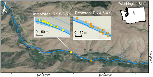
Individual growth data are useful in assessing relative habitat quality, but this approach is less common when evaluating the efficacy of habitat restoration. Furthermore, available models describing growth are infrequently combined with computational approaches capable of handling large data sets. We apply a mechanistic model to evaluate whether selection of restored habitat can affect individual growth. We used mark-recapture to collect size and growth data on sub-yearling Chinook salmon and steelhead in restored and unrestored habitat in five sampling years (2009, 2010, 2012, 2013, 2016). Modeling strategies differed for the two species: For Chinook, we compared growth patterns of individuals recaptured in restored habitat over 15-60 d with those not recaptured regardless of initial habitat at marking. For steelhead, we had enough recaptured fish in each habitat type to use the model to directly compare habitats. The model generated spatially explicit growth parameters describing size of fish over the growing season in restored vs. unrestored habitat. Model parameters showed benefits of restoration for both species, but that varied by year and time of season, consistent with known patterns of habitat partitioning among them. The model was also supported by direct measurement of growth rates in steelhead and by known patterns of spatio-temporal partitioning of habitat between these two species. Model parameters described not only the rate of growth, but the timing of size increases, and is spatially explicit, accounting for habitat differences, making it widely applicable across taxa. The model usually supported data on density differences among habitat types in Chinook, but only in a couple of cases in steelhead. Modeling growth can thus prevent overconfidence in distributional data, which are commonly used as the metric of restoration success.

Fig 1. Map of study area in the Entiat River.

Locations (river km relative to the confluence with the Columbia River) of the study reaches with restored pools and with unrestored pools are indicated.

Fig 2. Growth curves generated from Eq 1. over a 100 day growing period.

A: Effect of $\widehat{\alpha }$ on the timing of the inflection point. B: Effect of a on the slope of the growth curve. Panels C and D: Growth curves for values of the two parameters that are closer to those estimated from our data. For the curves in C in particular, the inflection point occurs close to time t = 0, so that the intercepts vary between parameter values. In these cases, fish are close to the lower bound on the curve Y′ when time is less than zero, which is to say, before sampling begins. In all panels Y′ = Y_∞ = 35.

Fig 3. Use of residual values (R) from a size vs. growth rate regression to compare growth in different habitats.

The arrow shows the distance from the points to the line. Mean residual values $\overline{R}$ are calculated for all individuals in each habitat (r = restored, u = unrestored), and if ${\overline{R}}_r>{\overline{R}}_u$, then we conclude that growth is higher in restored than in unrestored habitats.

Fig 4. Growth curves based on estimated model parameters (mean of the posterior) for Chinook salmon recaptured in treated habitat (“recaps,” solid lines) vs. those captured in either habitat type, but not recaptured (“others,” dashed lines).

The left panel shows the data and the habitat-specific models for all years combined. The small panels to the right show the data and the habitat-specific models for individual years. Parameter differences (see Fig 5) are shown in the upper left corner of each panel.

Fig 5. The difference (Δ; recaptures − others) in estimates of all model parameters ± the 95% credible interval between the two capture types of young-of-the-year Chinook salmon.

Recaptures in restored habitat; others = fish marked and not recaptured, regardless of capture origin. Year-specific estimates incorporate the random effect of year, and combined differences are based on the average parameter values among years. The number in parentheses represents the fraction of posterior draws for which the difference was above or below zero, as appropriate. Δ Length at time = 0 was substituted for model parameter Y′.

Fig 6. Growth curves based on estimated model parameters (mean of the posterior) for steelhead recaptured in restored habitat (solid lines) vs. those recaptured in unrestored habitat (dashed lines).

Left panel shows data and fitted curves for all years combined; additional figures show individual years. Parameter differences (see Fig 7) are indicated in the lower right corner of each panel. The analysis omits 2013 owing to lack of long-term steelhead recaptures in unrestored habitats.

Fig 7. The difference in estimates of all model parameters ± the 95% credible interval between the two capture types of young-of-the-year steelhead (recaptures in restored habitat—recaptures in unrestored habitat).

Year-specific estimates incorporate the random effect of year, and combined differences are based on the average parameter values among years. The number in parentheses represents the fraction of posterior draws for which the difference was above or below zero, depending on trend of the data. For all panels except the lower right, this represents the fraction of posterior draws above zero. Δ Length at time = 0 was substituted for model parameter Y′. The analysis omits 2013 owing to lack of long-term steelhead recaptures in unrestored habitats.

Fig 8. Mean residuals from a log-linear regression of growth rate versus size, in restored vs. unrestored habitat, for each study year.

The analysis omits 2013 owing to lack of long-term steelhead recaptures in unrestored habitats.

References

1. Taylor BL, Wade PR. “Best” abundance estimates and best management: why they are not the same Quantitative methods for conservation biology Springer-Verlag, New York, New York, USA: 2000; p. 96–108.
1. Irwin LL, Rock DF, Rock SC, Loehle C, Van Deusen P. Forest ecosystem restoration: Initial response of spotted owls to partial harvesting. Forest Ecology and Management. 2015;354:232–242. 10.1016/j.foreco.2015.06.009 - DOI
1. Sievers M, Hale R, Morrongiello JR. Do trout respond to riparian change? A meta-analysis with implications for restoration and management. Freshwater Biology. 2017;62(3):445–457. 10.1111/fwb.12888 - DOI
1. Morris WF, Doak DF, et al. Quantitative conservation biology. Sinauer, Sunderland, Massachusetts, USA: 2002.
1. Scheuerell MD, Hilborn R, Ruckelshaus MH, Bartz KK, Lagueux KM, Haas AD, et al. The Shiraz model: a tool for incorporating anthropogenic effects and fish–habitat relationships in conservation planning. Canadian Journal of Fisheries and Aquatic Sciences. 2006;63(7):1596–1607. 10.1139/f06-056 - DOI
Publication types