Asexual Evolution and Forest Conditions Drive Genetic Parallelism in Phytophthora ramorum

Abstract

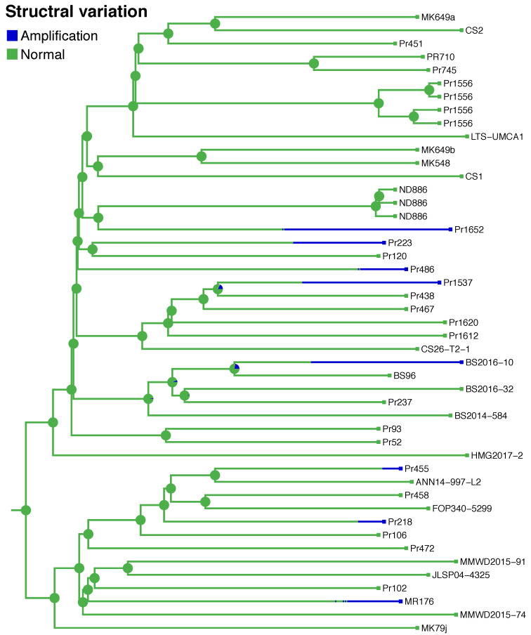
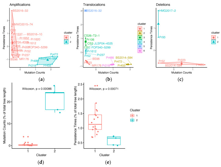
It is commonly assumed that asexual lineages are short-lived evolutionarily, yet many asexual organisms can generate genetic and phenotypic variation, providing an avenue for further evolution. Previous work on the asexual plant pathogen Phytophthora ramorum NA1 revealed considerable genetic variation in the form of Structural Variants (SVs). To better understand how SVs arise and their significance to the California NA1 population, we studied the evolutionary histories of SVs and the forest conditions associated with their emergence. Ancestral state reconstruction suggests that SVs arose by somatic mutations among multiple independent lineages, rather than by recombination. We asked if this unusual phenomenon of parallel evolution between isolated populations is transmitted to extant lineages and found that SVs persist longer in a population if their genetic background had a lower mutation load. Genetic parallelism was also found in geographically distant demes where forest conditions such as host density, solar radiation, and temperature, were similar. Parallel SVs overlap with genes involved in pathogenicity such as RXLRs and have the potential to change the course of an epidemic. By combining genomics and environmental data, we identified an unexpected pattern of repeated evolution in an asexual population and identified environmental factors potentially driving this phenomenon.

Keywords: Phytophthora ramorum; Structural Variants; asexual reproduction; forest pathology; parallel evolution.

Figure 1

Maps of California counties where P. ramorum isolates were collected. Longitude and latitude are shown on the x- and y-axis. (a) Left panel shows the counties outlined in white where isolates used in the phylogeny (Figure 2, and Figure 4) were collected. Red triangles refer to Sonoma Co. and Monterey Co. which are zoomed in on the (b) top right and (c) bottom right panels. Red circles indicate plots where non-wild type (NWT) isolates were collected, and blue circles show where wild type (WT) isolates were collected. Isolates collected from (b) Sonoma Co. and (c) Monterey Co. plots where used in the environmental association study (Figure 6).

Figure 2

Phylogenetic reconstruction of P. ramorum NA1 in California. (a) Splitstree graph using SNPs indicates resolved relationships and discordances as links between branches; (b) phylogeny using BEAST v1.8.0 under the Birth–Death serial sample model. Node labels are the posterior probabilities of node height and line color represent posterior support of SNP mutation rate. Isolate identification numbers are followed by the California county of origin and naming conventions are consistent with previous publications. The first letters of the identification number represent the original project or the collector (e.g., BS = Big Sur project, and MMWD = Marin Municipal Water District). Pr1556 and ND886 served as controls during sequencing and the dates following their name indicate the time they were sequenced (e.g., August 2017).

Figure 2

Phylogenetic reconstruction of P. ramorum NA1 in California. (a) Splitstree graph using SNPs indicates resolved relationships and discordances as links between branches; (b) phylogeny using BEAST v1.8.0 under the Birth–Death serial sample model. Node labels are the posterior probabilities of node height and line color represent posterior support of SNP mutation rate. Isolate identification numbers are followed by the California county of origin and naming conventions are consistent with previous publications. The first letters of the identification number represent the original project or the collector (e.g., BS = Big Sur project, and MMWD = Marin Municipal Water District). Pr1556 and ND886 served as controls during sequencing and the dates following their name indicate the time they were sequenced (e.g., August 2017).

Figure 3

Processes that lead to genetic variants include somatic mutations and recombination. Three hypothetical scenarios are shown: (a) Normal state [no Structural Variants (SVs)]; (b) SV arising from somatic mutation; and (c) genetic variation (arising from recombination between individuals). Three individuals are represented (e.g., Ind 1, 2, and 3) and their corresponding haplotypes (H1 and H2). Haplotypes: H1, black; H2, white. Green brackets, genomic regions with variation; red lines, hypothetical SNPs that distinguish haplotypes. (b) Individuals with somatic SVs (e.g., amplification, assuming duplication occurs by tandem duplication) show an increase in haplotype (H1H1/H2, H1/H2H2, or H1H1/H2H2). (c) Genetic variants from recombination are likely to have allele combinations representing genotypes found in a Hardy–Weinberg equation (i.e., H1/H1, H1/H2, and H2/H2).

Figure 4

Ancestral state reconstruction of SVs indicates patterns of parallelism and estimates of persistence time. Example phylogeny testing duration of persistence time comes from SV117. The legend in the top left corner indicates the SV type (blue for amplifications, and green for normal state). The branch lengths correspond to time in years. Branches leading to Pr1652, Pr1537, and BS2016-10 had longer persistence times in the amplification state compared to branches leading to Pr223, Pr486, Pr455, Pr218, and MR176. Pie charts at each internal node indicate the posterior estimate of the SV ancestral state.

Figure 5

SV persistence times and mutation counts of isolates. K-means clustering grouped isolates with SVs into (a) two groups of amplifications, (b) six groups of translocations, and (c) two groups of deletions. Each point represents an isolate with their corresponding persistence time (scaled by branch length) vs. mutation count. Numbers of clusters were determined by the Silhouette Method. Significant differences in mutation counts (d) and persistence times (e) were examined for the two clusters in the K-means analysis of amplifications. The two clusters of amplifications represent isolates with higher persistence times (1.1%) and lower mutation counts (0.2, Cluster 1), and isolates with lower persistence times (0.7%) and higher mutation counts (24.1, Cluster 2).

Figure 6

Correlation coefficients between forest environmental factors and genetic parallelism or phenotype. Posterior parameter estimates from Bayesian generalized linear hurdle Poisson models of parallel SVs in response to Jaccard’s distance of environmental factors (a). Posterior parameter estimates from a generalized linear model with a Bernoulli distribution (logit link function) of Jaccard’s distance between environmental conditions associated with NWT phenotype (b). Jaccard distance of environmental variables are calculated as the difference between Monterey Co. and Sonoma Co. First model (top panels) includes minimum temperature of the coldest month (bio 6), precipitation of the coldest quarter (bio19), N. densiflorus and U. californica stem density (LIDE.UMCA), precipitation during Spring (Springppt), Elevation, and a hurdle probability (hu). Second model (bottom panels) includes the same parameters, except solar radiation during August (sun radiation Aug) replaces minimum temperature during the coldest month. Bayes factor comparing both models was not significant (1.66).

References

1. Martin F.N., Tooley P.W. Phylogenetic relationships of Phytophthora ramorum, P. nemorosa, and P. pseudosyringae, three species recovered from areas in California with sudden oak death. Mycol. Res. 2003;107:1379–1391. doi: 10.1017/S0953756203008785. - DOI - PubMed
1. Omilian A.R., Cristescu M.E.A., Dudycha J.L., Lynch M. Ameiotic recombination in asexual lineages of Daphnia. Proc. Natl. Acad. Sci. USA. 2006;103:18638–18643. doi: 10.1073/pnas.0606435103. - DOI - PMC - PubMed
1. Schwander T., Crespi B.J. Multiple Direct Transitions from Sexual Reproduction to Apomictic Parthenogenesis in Timema Stick Insects. Evolution. 2009;63:84–103. doi: 10.1111/j.1558-5646.2008.00524.x. - DOI - PubMed
1. Oxley P.R., Ji L., Fetter-Pruneda I., McKenzie S.K., Li C., Hu H., Zhang G., Kronauer D.J.C. The genome of the clonal raider ant. Cerapachys biroi. Curr. Biol. CB. 2014;24:451–458. doi: 10.1016/j.cub.2014.01.018. - DOI - PMC - PubMed
1. Seidl M.F., Thomma B.P.H.J. Sex or no sex: Evolutionary adaptation occurs regardless. BioEssays. 2014;36:335–345. doi: 10.1002/bies.201300155. - DOI - PMC - PubMed