Agent-Based Models Predict Emergent Behavior of Heterogeneous Cell Populations in Dynamic Microenvironments

Abstract

Computational models are most impactful when they explain and characterize biological phenomena that are non-intuitive, unexpected, or difficult to study experimentally. Countless equation-based models have been built for these purposes, but we have yet to realize the extent to which rules-based models offer an intuitive framework that encourages computational and experimental collaboration. We develop ARCADE, a multi-scale agent-based model to interrogate emergent behavior of heterogeneous cell agents within dynamic microenvironments and demonstrate how complexity of intracellular metabolism and signaling modules impacts emergent dynamics. We perform in silico case studies on context, competition, and heterogeneity to demonstrate the utility of our model for gaining computational and experimental insight. Notably, there exist (i) differences in emergent behavior between colony and tissue contexts, (ii) linear, non-linear, and multimodal consequences of parameter variation on competition in simulated co-cultures, and (iii) variable impact of cell and population heterogeneity on emergent outcomes. Our extensible framework is easily modified to explore numerous biological systems, from tumor microenvironments to microbiomes.

Keywords: agent-based model; cell population dynamics; computational modeling; emergent behavior; microenvironment.

Figure 1

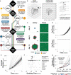
Overview of agent-based model framework. (A) Diagram of package structure and interfaces. Agents include Cell, Module, and Helper and environments include Grid, Lattice, Component, and Location. By importing an interface, a class is guaranteed a certain set of methods with which it can interact with objects of the imported interface. (B) Interfaces can be implemented into concrete classes in a variety of ways, depending on the system of interest. Classes with solid border are implemented in our model. (C) Overview of the modeling pipeline. Inputs, defined with an XML (.xml) file, are parsed to create a simulation series. Within the simulation series, for each random seed, a simulation instance is created. Environments and agents are added to the simulation instance. The simulation is stepped, and data is output to a JSON (.json) file. Alternatively, the simulation can be run in GUI mode.

Figure 2

Tissue cell implementation. (A) Flowchart outlining tissue cell agent states and the rules governing transitions between them at each tick of the simulation. (B) Diagram of the simulation environment structure comprising a hexagonal grid for cells and triangular lattices for molecules. Environment size is defined by radius R from the center hexagon and a margin M between the cell grid and the molecule lattices. For 3D simulations, layers of 2D simulations are stacked at a height H from the center layer. (C) Spatial distribution of cell states for colony (left) and tissue (right) growth for a single example replicate (random seed 0) at different timepoints during the simulation. Scale bars represent 100 μm. (D) Plot of total cell count for colony (top) and tissue (bottom) growth for each of n = 50 replicate simulations of the model with default parameters and settings. Each line shows the trajectory for a single simulation. (E) Plot of average colony diameter for each of n = 50 replicate simulations of the model with default parameters and settings. Each line shows the trajectory for a single simulation. Dashed and dotted lines indicate experimentally observed diameters (Conger and Ziskin, ; Brú et al., 2003), respectively. (F) Violin plots of doubling times for the simulation (n = 50) calculated using (i) cell count doublings at t = 7 days and (ii) exponential curve fit to the first 7 days of growth compared to doubling times of the cancer cell lines in the NCI-60 panel (Alley et al., 1988), both aggregated and separated by pathology. Black circle indicates mean. (G) Scatter plot of colony diameter and number of cells in the colony for colonies less than 160 μm in diameter across n = 50 replicate simulations. Solid lines show the relationship between colony diameter, number of cells in the colony, and diameter of a colony cell using an equation fit to experimental data (Meyskens et al., 1984). Dotted lines show the same relationship for an equation of the same form fit to the simulation results. Colors indicate the difference between the cell diameter calculated directly from the simulation data and the cell diameter predicted by the experimental fit.

Figure 3

Metabolism and signaling module complexity. (A) Diagram summarizing the differences between complexities of the metabolism module. All modules uptake glucose (G) and oxygen (O) from the environment through various mechanisms. Cell size regulation by autophagy is indicated by dotted ring. Only complex metabolism explicitly accounts for a pyruvate (P) intermediate. Nutrient uptake can be variable (solid, black arrow), constant (solid, empty arrow), or random (dotted, gray arrow). (B) Diagram summarizing the differences between complexities of the signaling module. The non-random modules interact with extracellular TGFα (T). Number of rings indicate how many cellular compartments (i.e., membrane, cytoplasm, and/or nucleus) are explicitly included in the signaling network. Large dots denote molecular species within the network and small dots denote regulatory interactions. (C) Time course of growth rate, symmetry, and cycle length for different complexities of the metabolism and signaling modules, grouped by signaling module complexity. (D) Distribution of cell states as a function of distance from the center of the colony at t = 2 weeks. Solid line, dotted line, and shaded area denote the mean, standard deviation, and range across n = 20 replicates. Light gray rectangle is a visual reference for a distance of 0.3 mm from the center across all cell states.

Figure 4

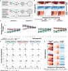
Case study 1: Context. (A) Diagram of the three sets of simulations. First, three parameters at the cell, metabolism, and signaling scales (crowding tolerance, metabolic preference, and migratory threshold, respectively) were varied +/− 100% (increments of 10%) and initialized onto an empty environment. Second, combinations of representative cell populations (A, B, C, and X) were initialized onto an empty environment to represent a colony context. Third, combinations of representative cell populations (A, B, C, and X) were initialized onto an environment containing a generic cell population to represent a tissue context. (B) Sensitivity of three metrics to variation in the three parameters calculated as (y − y₀)x₀/(x − x₀)y₀ where y is the metric value and x is the parameter value. Circle size indicates relative fold change in sensitivity to the maximum for a given metric and parameter, circle color indicates absolute sensitivity, and inverse relationships are indicated by a black border. (C) Relative change in population fraction for each of the four representative populations over time across all combinations under colony and tissue contexts. Color indicates the other populations included in the simulation; black indicates all three other populations where included. (D) Time course of metric values for the four representative populations under colony and tissue contexts. Violin plots show distribution of the metric value between contexts at time t = 2 weeks for all population combinations (^*) or for population combinations including the indicated population. (E) Heat map of the change in metric value between the (colony) − (tissue) contexts at different timepoints for all population combinations.

Figure 5

Case study 2: Competition. (A) Diagram of the set of simulations. Three parameters at the cell, metabolism, and signaling scales (crowding tolerance, metabolic preference, and migratory threshold, respectively) were varied +/− 50% (increments of 10%) and initialized in ratios of 0 to 100% (increments of 10%) with a basal, unmodified cell population onto an empty environment. (B) Relative change in population fraction for the modified population over time for different changes in parameter at selected initial ratios of the modified population. (C) Heat maps of fold change in metric value across n = 20 replicates for different changes in parameter and initial ratios relative to a 0% change in parameter at t = 2 weeks. (D) Spatial distribution of change in fraction of the modified population at t = 2 weeks across n = 20 replicates for simulations initialized with an equal mixture of the modified and basal cell populations. Locations with less than 0.5 fraction occupancy across replicates are shown in gray.

Figure 6

Case study 3: Heterogeneity. (A) Diagram of the two sets of simulations. First, combinations of representative cell populations (A, B, C, and X) with heterogeneity H varied at 0, 10, 20, 30, 40, and 50% were initialized onto an empty environment to represent a colony context. Second, combinations of representative cell populations (A, B, C, and X) with heterogeneity H varied at 0, 10, 20, 30, 40, and 50% were initialized onto an environment containing a generic cell population with background heterogeneity H₀ varied at 0, 10, 20, 30, 40, and 50% to represent a tissue context. (B) Heat maps of fold change in metrics for each representative cell population across different amounts of heterogeneity relative to the non-heterogeneous (H = 0) case at t = 2 weeks. The colony context (no background population) is indicated by the bullet (•). (C) Relative change in population fraction for each of the four representative populations for all combinations as a function of heterogeneity at t = 2 weeks. Color indicates the other populations included in the simulation; black indicates all three other populations where included. Lines connect average values for the colony context (thin) and averages across values for different background heterogeneities for the tissue context (thick) for each combination. (D) Distributions parameter means across n = 20 replicates at different timepoints under colony and tissue contexts for representative cell populations with H = H₀ = 40. (E) Heat maps of change in metric value between the (colony with heterogeneity) – (tissue with heterogeneity) contexts for representative cell populations at t = 2 weeks.

References

1. Abercrombie M., Heaysman J. E. (1953). Observations on the social behaviour of cells in tissue culture. Exp. Cell Res. 5, 111–131. 10.1016/0014-4827(53)90098-6 - DOI - PubMed
1. Alley M. C., Scudiero D. A., Monks A., Hursey M. L., Czerwinski M. J., Fine D. L., et al. . (1988). Feasibility of drug screening with panels of human tumor cell lines using a microculture tetrazolium assay. Cancer Res. 48, 589–601. - PubMed
1. Altschuler S. J., Wu L. F. (2010). Cellular heterogeneity: do differences make a difference? Cell 141, 559–563. 10.1016/j.cell.2010.04.033 - DOI - PMC - PubMed
1. An G., Mi Q., Dutta-Moscato J., Vodovotz Y. (2009). Agent-based models in translational systems biology. Wiley Interdiscipl. Rev. Syst. Biol. Med. 1, 159–171. 10.1002/wsbm.45 - DOI - PMC - PubMed
1. Athale C., Mansury Y., Deisboeck T. S. (2005). Simulating the impact of a molecular ‘decision-process’ on cellular phenotype and multicellular patterns in brain tumors. J. Theor. Biol. 233, 469–481. 10.1016/j.jtbi.2004.10.019 - DOI - PubMed
LinkOut - more resources