Vibrational Spectroscopic Map, Vibrational Spectroscopy, and Intermolecular Interaction

Abstract

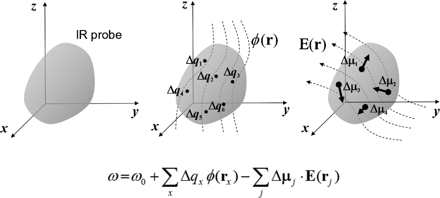
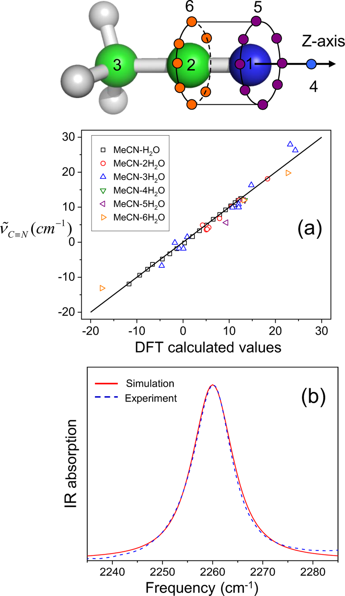
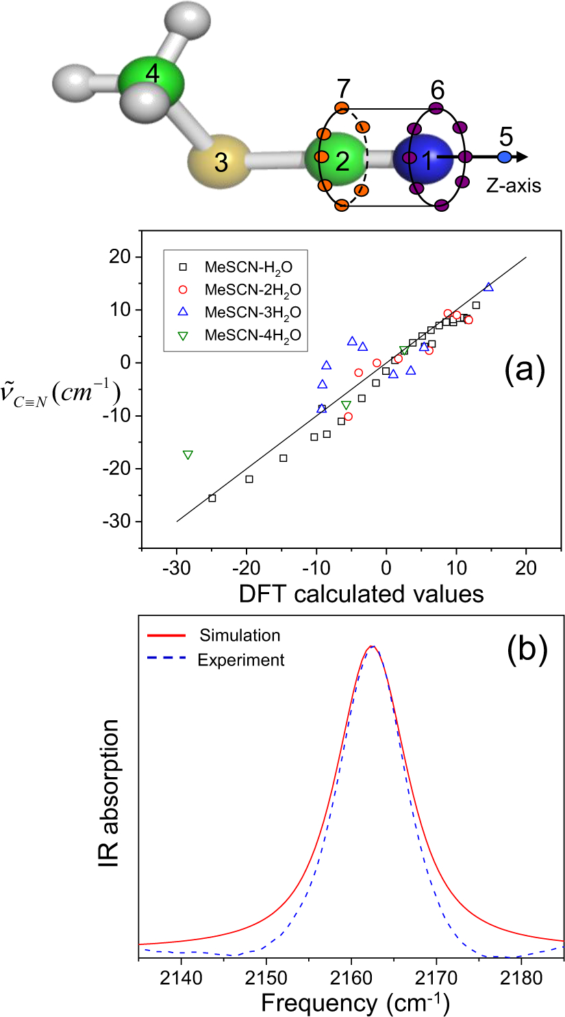
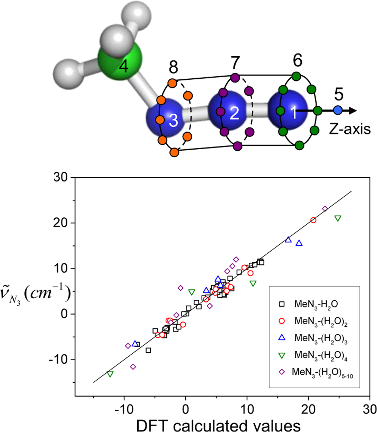
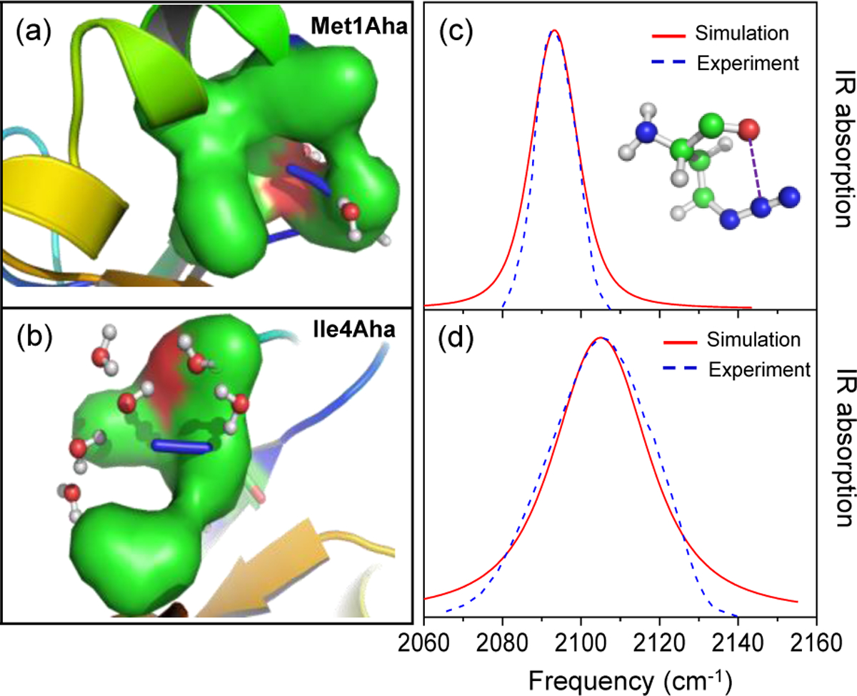
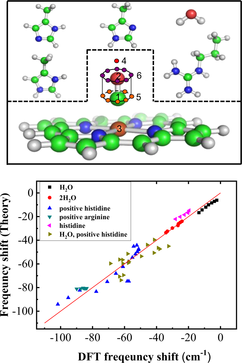
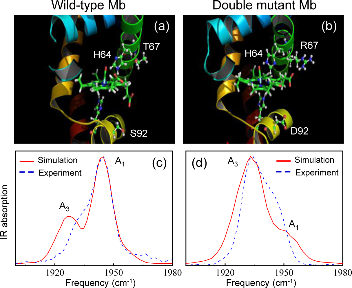
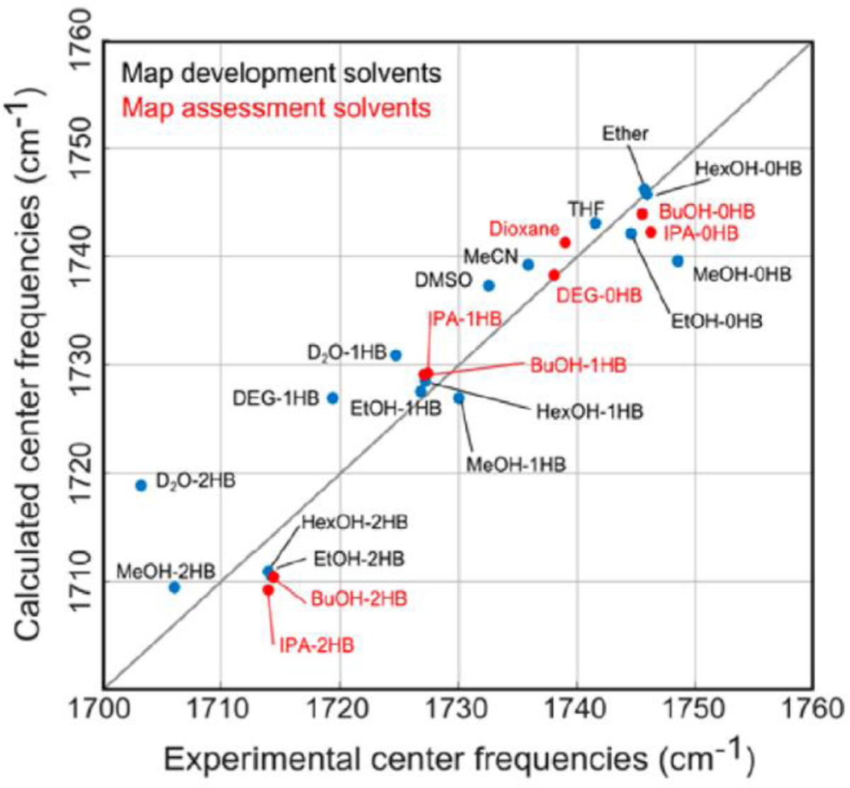
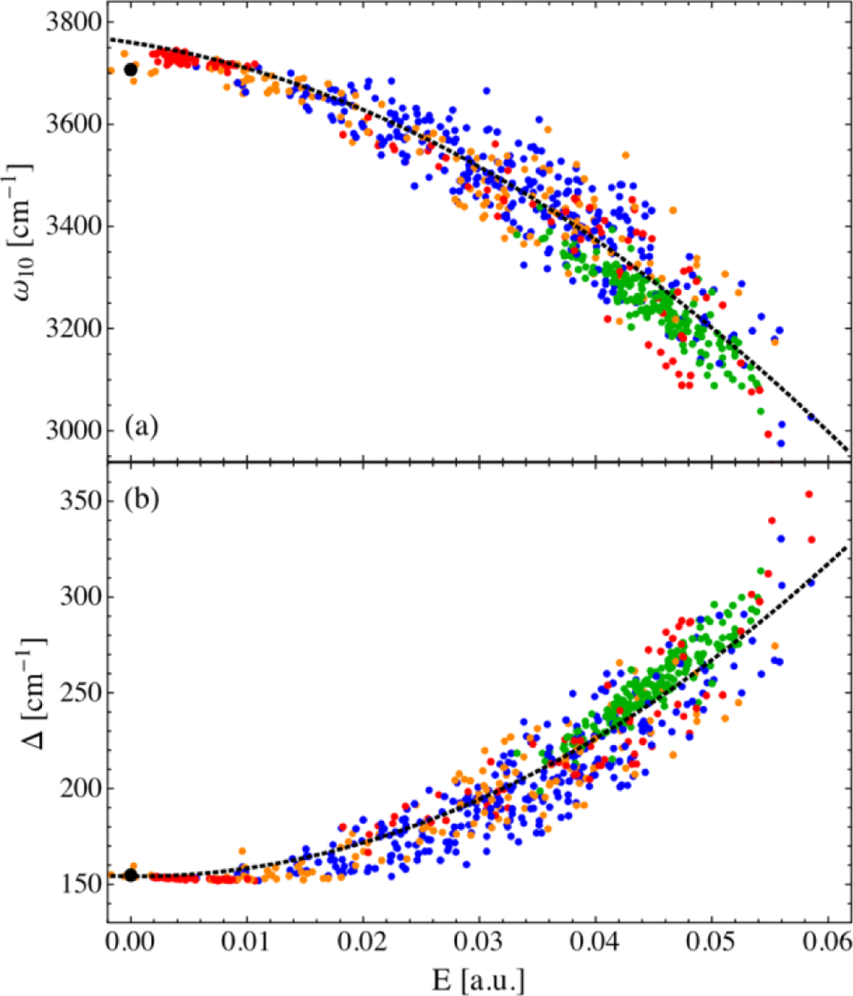
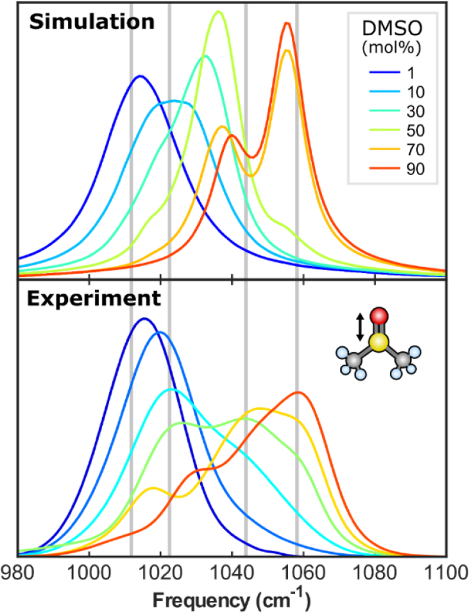
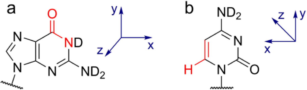
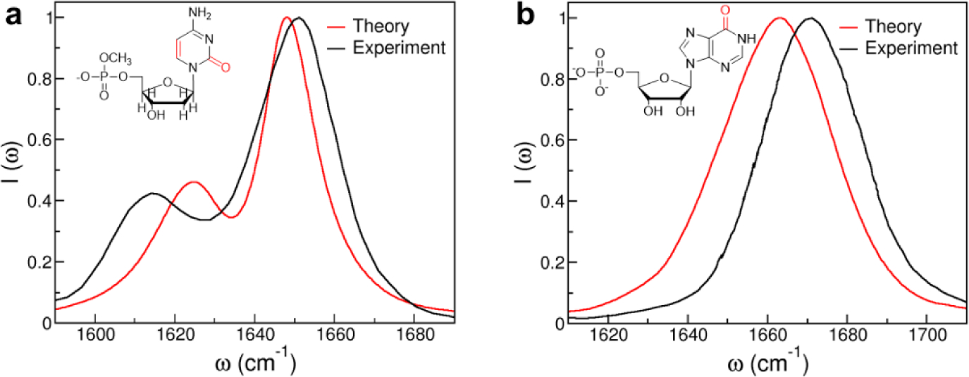
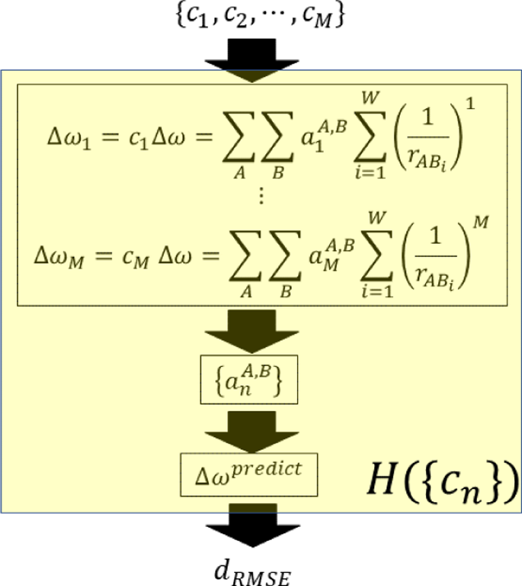
Vibrational spectroscopy is an essential tool in chemical analyses, biological assays, and studies of functional materials. Over the past decade, various coherent nonlinear vibrational spectroscopic techniques have been developed and enabled researchers to study time-correlations of the fluctuating frequencies that are directly related to solute-solvent dynamics, dynamical changes in molecular conformations and local electrostatic environments, chemical and biochemical reactions, protein structural dynamics and functions, characteristic processes of functional materials, and so on. In order to gain incisive and quantitative information on the local electrostatic environment, molecular conformation, protein structure and interprotein contacts, ligand binding kinetics, and electric and optical properties of functional materials, a variety of vibrational probes have been developed and site-specifically incorporated into molecular, biological, and material systems for time-resolved vibrational spectroscopic investigation. However, still, an all-encompassing theory that describes the vibrational solvatochromism, electrochromism, and dynamic fluctuation of vibrational frequencies has not been completely established mainly due to the intrinsic complexity of intermolecular interactions in condensed phases. In particular, the amount of data obtained from the linear and nonlinear vibrational spectroscopic experiments has been rapidly increasing, but the lack of a quantitative method to interpret these measurements has been one major obstacle in broadening the applications of these methods. Among various theoretical models, one of the most successful approaches is a semiempirical model generally referred to as the vibrational spectroscopic map that is based on a rigorous theory of intermolecular interactions. Recently, genetic algorithm, neural network, and machine learning approaches have been applied to the development of vibrational solvatochromism theory. In this review, we provide comprehensive descriptions of the theoretical foundation and various examples showing its extraordinary successes in the interpretations of experimental observations. In addition, a brief introduction to a newly created repository Web site (http://frequencymap.org) for vibrational spectroscopic maps is presented. We anticipate that a combination of the vibrational frequency map approach and state-of-the-art multidimensional vibrational spectroscopy will be one of the most fruitful ways to study the structure and dynamics of chemical, biological, and functional molecular systems in the future.

Figure 1.

Vibrational frequency mapping with solvent electric potential and field. The vibrational frequency ω of a normal mode of an IR probe is mapped onto a set of points, called distributed sites, that interact with the electrostatic potential ϕ and electric field E exerted by the molecular environment. Note that the map parameters Δq_x, which are vibrational solvatochromic charges, are scalar quantities whereas Δμ_x, which are vibrational solvatochromic dipoles, are Cartesian vectors. The vibrational reference frequency, ω₀, which could also be a part of the map, corresponds to that of the IR probe in the absence of solvent electrostatic potential and electric field.

Figure 2.

Schematic diagram of the 2D IR spectra of two oscillators. The x and y axes represent the excitation (pump) and emission (probe) frequencies, respectively. Here, it should be mentioned that sometimes 2D spectra are plotted with the two axes swapped. Two diagonal peaks with positive (red) amplitudes originate from the ground-state bleach and stimulated emission, whereas those with negative (blue) amplitudes are from the excited-state absorption. The center line slope (CLS) and nodal line slope (NLS) are related to the frequency-frequency correlation function and the inhomogeneity of the transition frequencies. If the two oscillators are coupled with each other via wave function overlap, one can find cross-peaks at zero waiting time. If the two oscillators exchange energy or undergo chemical exchange, the cross-peaks in the off-diagonal region of the 2D IR spectrum appear as the waiting time, T_w, increases.

Figure 3.

Left: Nitrile stretching mode frequencies of acetonitrile (MeCN, closed squares) and methyl thiocyanate (MeSCN, open circles) plotted with respect to the hydrogen-bond angle, θ, between the nitrile’s N atom and the hydrogen atom of the H-bonded water molecule. Reproduced from Figure 2 of Ref. Copyright 2008 AIP Puplishing. Right: Experimentally measured mean nitrile vibrational frequency plotted with respect to the average value of θ from MD simulations of nine variants of GFP containing p-cyanophenylalanine (given in the figure key). Reproduced from Figure 8(B) of Ref. Copyright 2018 The American Chemical Society.

Figure 4.

(a) Summary of the models used for spectral calculations. Parametrized sites are shown in red. The red shading in the MF model schematically indicates the transition charge region for sampling. Cho-Potential model 1 (CP1) utilized parametrized partial charges whereas other models utilize partial charges defined in MD simulations. Knoester-Field model 1 (KF1) utilized NNFS maps. (b) The amide-I local mode frequency shifts calculated with the six models for the restrained trajectory. Blue circles: solvent contributions $\left(\overline{\delta {\omega }_{i,\text{S}}}\right)$; red circles: peptide backbone and side-chain contributions $\left(\overline{\delta {\omega }_{i,\text{P}}}\right)$; black circles: total shifts $\left(\overline{\delta {\omega }_i}\right)$. The vertical bars indicate the range enclosed by ± one standard deviation (σ_i). Green symbols with solid and dash lines in KF1 are the NNFS and electrostatic contributions in $\overline{\delta {\omega }_{i,\text{P}}}$, respectively. Reproduced from Table 1 and Figure 8 of Ref. Copyright 2009 The American Chemical Society.

Figure 5.

The linear and 2D IR spectra calculated with the CP1, CP2, KP, KF1, KF2, and MF models for the restrained trajectory. The number in the upper right corner of the FT IR spectrum panel indicates the frequency shift (in cm⁻¹) applied to the calculated spectra. Red and black lines in the linear spectra correspond to the simulated and experimental data, respectively. Reproduced from Figure 7 of Ref.. Copyright 2009 The American Chemical Society.

Figure 6.

Structure and 2D IR spectra of isotope-labeled hIAPP from reference. The sequence (A) and structural model (B) of hIAPP with the ¹³C=¹⁸O isotope labels highlighted. 2D IR spectra and the diagonal intensity slices of the lag-phase and equilibrium phase V17 (C sand D) and F23 (E and F) labeled proteins. The boxes and arrows indicate the ¹³C=¹⁸O labeled modes. Reproduced from Figure 1 of Ref. Copyright 2013 the National Academy of Sciences of the United States of America.

Figure 7.

(A) Sequence of the macrocycle with the isotope labeled positions highlighted. (B) Comparison of experimental and theoretical 2D IR line widths. The theoretical spectra are calculated using various coupling schemes. Reproduced from Figure 1A and Figure 6 of Ref. Copyright 2012 American Chemical Society.

Figure 8.

(Taken from Figure 8 of Ref) Comparison of the frequencies, line widths, and intensities of experimental spectra with simulated spectra starting from MD simulations of the crystal structure of the protein G mutant NuG2b. Copyright 2016 Annual Reviews.

Figure 9.

Molecular structures of alanine dipeptide in the upper panel. IR and VCD spectra of amide I, II, and III modes are displayed for its RHH and P_II conformations in the bottom panel. The blue solid and red dashed lines correspond to the simulated spectra obtained from DFT calculation and the fragment approximation, respectively. Reproduced from Figures 1, 3, and 4 of Ref.. Copyright 2009 Elsevier.

Figure 10.

Nearest-neighbor amide I/I, I/II, II/I, and II/II coupling maps calculated for AcGlyNHMe at the B3LYP/6–31+G(d) level with fixed dihedral angles. All four maps are plotted in a single color scale and the unit of couplings is cm⁻¹. Reproduced from Figure 8 of Ref.. Copyright 2009 The American Chemical Society.

Figure 11.

Experimental (black) and simulated (red) linear IR spectra of a 3₁₀-helical hexapeptide Z-Aib-L-Leu-(Aib)₂-Gly-OtBu in CDCl₃ in the amide I and II regions. B1, B2, and B3 are six-site potential models, K is a four-site field/gradient model, G is a four-site potential model, and Em is a semiempirical model. The local amide I frequency was shifted from the gas phase value by the value reported in each panel. Reproduced from Figure 8 of Ref.. Copyright 2010 The American Chemical Society.

Figure 12.

Experimental and simulated absolute 2D IR rephasing (top) and nonrephasing (bottom) spectra of a 3₁₀-helical hexapeptide Z-Aib-L-Leu-(Aib)₂-Gly-OtBu in the amide II frequency region. Each spectrum is normalized by the peak intensity of the diagonal amide II band. Reproduced from Figure 10 of Ref.. Copyright 2010 The American Chemical Society.

Figure 13.

Solvatochromic charge model with distributed interaction sites for MeCN in the upper panel. The calculated nitrile stretching mode frequency shift using Eq. (109) is directly compared to the DFT calculation results in (a). The numerically simulated IR spectrum of the CN stretch mode (solid red line) is plotted with the experimentally measured result (blue dashed line) in (b). The figure of the interaction sites and (a) is reproduced from Figure 5(a) Ref. and (b) is reproduced from Figure 10(a) of Ref.. Copyright 2008 AIP Puplishing.

Figure 14.

Solvatochromic charge model with distributed interaction sites for MeSCN in the upper panel. The y-axis in (a) corresponds to the thiocyanato stretch mode frequency obtained with Eq. (109) and the x-axis to the DFT calculated results. The numerically simulated IR spectrum of the SCN stretch mode (red solid line) is plotted with the experimentally measured result (blue dashed line) in (b). The figure of the interaction sites and (a) is reproduced from Figure 5(b) of Ref. and (b) is reproduced from Figure 10(b) of Ref.. Copyright 2008 AIP Puplishing.

Figure 15.

Solvatochromic charge model with distributed interaction sites for MeN₃ in the upper panel. The y-axis in the bottom panel represents the azido stretch mode frequency obtained with Eq. (109) and the x-axis to the DFT calculated results. Reproduced from Figures 4(b) and 5 of Ref.. Copyright 2008 AIP Puplishing.

Figure 16.

(a) Azido group in the hydrophobic pocket of Met1Aha NTL9 mutant (b) fully hydrated azido group of Ile4Aha NTL9 mutant. The numerically calculated IR spectra of the azido stretch mode (solid red line) of Met1Aha in (c) and Ile4Aha in (d) are displayed with the experimental results (blue dashed line). Reproduced from Figures 1 and 4 of Ref.. Copyright 2011 The American Chemical Society.

Figure 17.

The heme-CO complex, a distributed solvatochromic charge model of the top panel, is shown along with model compounds such as neutral histidine, positively charged histidine protonated at the atom of N_ε or N_δ, positively charged arginine and water molecules. In the bottom panel, the frequency shift of the CO stretch mode theoretically obtained from the Eq. (109) is compared with the DFT calculation result. Reproduced from Figures 1 and 2 of Ref.. Copyright 2013 The American Chemical Society.

Figure 18.

(a) Protein structures obtained from MD simulation of native MbCO in (a) and the double mutant MbCO in (b). The double mutant has two substituted residues of Arg67 (R67) and Asp92 (D92) instead of Thr67 (T67) and Ser92 (S92) in the wild type. The numerically calculated IR spectra of the CO stretch mode (solid red line) of native MbCO in (c) and the double mutant in (d) are displayed with the experimental results (blue dashed line). Reproduced from Figures 4 and 9 of Ref.. Copyright 2013 The American Chemical Society.

Figure 19.

Comparison between computed and experimental CO center frequencies and line widths in all solvents. Solvents used to parametrize the map are indicated in blue, and solvents used to evaluate the map performance are shown in red. The solvents are labeled Ether = diethyl ether, THF = tetrahydrofuran, MeCN = acetonitrile, HexOH = hexanol, EtOH = ethanol, MeOH = methanol, BuOH = butanol, IPA = isopropanol, and DEG = diethylene glycol. Reproduced from Figure 7 of Ref.. Copyright 2016 The American Chemical Society.

Figure 20.

Reproduced with permission from Figure 2 of Ref.. (a) DFT calculations of the OH stretch vibrational frequency, ω₁₀, of HOD in various environments, including (black) a gas-phase monomer, (red) a water hexamer at 80 K, (blue) liquid water, (green) ice I_h at 100 K, and (orange) the water/vacuum interface. The dashed line is a spectroscopic map in terms of the electric field, E, along the OH bond evaluated at the site of the H atom. (b) Calculated anharmonicity, Δ, of the OH vibration. Copyright 2013 The American Chemical Society.

Figure 21.

Experimental and computed IR absorption spectra of the S=O stretching mode at different concentrations in binary DMSO/water mixtures. Computed spectra were obtained using the map of Oh and Baiz. Vertical bars represent the average experimental frequencies of the four DMSO species present in solution: singly hydrogen-bonded (1HB), doubly-hydrogen bonded (2HB), Aggregate (Agg), and non-hydrogen bonded (Free) from low to high frequency respectively. Adapted from Figure 1 of Ref. Copyright 2019 AIP Puplishing.

Figure 22.

Coordinate systems of the (a) C=O and (b) C=C vibrational frequency maps. The atoms used to define the axes are shown in red. Reproduced from Figure 4 of Ref.. Copyright 2019 The American Chemical Society.

Figure 23.

Theoretical and experimental^, IR spectra of (a) deoxycytidine 5’-monophosphate and (b) inosine 5’-monophosphate in D₂O. The chemical structures of the molecules are shown in the insets with their chromophores highlighted in red. Reproduced from Figure 7 and Figure 9 of Ref.. Copyright 2019 The American Chemical Society.

Figure 24.

Schematic diagram of the procedure from the relative contributions c_n to the RMSE value, d_RMSE.

Figure 25.

(a-d) Magnitude of relative contributions c_i when we use as a training set (a) 1W, (b) 2–5W, (c) 6–35W, and (d) 50W set. (e) Relative contributions c_i for the training set of the study in Ref. Reproduced from Figure 10 of Ref.. Copyright 2019 AIP Puplishing.

Figure 26.

RMSE in transition frequency and dipole derivative of the OH-stretch (blue line) local mode depending on which atoms’ local chemical environment is used as an input to ANN (marked in red). The leftmost set of bars corresponds to RMSEs of the spectroscopic maps developed in Ref, all others correspond to the Δ -ML approach of ref. (Adapted from Figure 2 of Ref.) Copyright 2019 The American Chemical Society.

Figure 27.

The plot of the training and the validation RMSE values as a function of elapsed epochs in the training of the feed forward neural network model with the unscaled terms of the polynomial function. Adapted from Figures 7 and 8(a) of Ref. Copyright 2020 AIP Puplishing.

References

1. Herzberg G Molecular Spectra and Molecular Structure I: Spectra of Diatomic Molecules; Van Nostrand, 1950.
1. Herzberg G Molecular Spectra and Molecular Structure II: Infrared and Raman of Polyatomic Molecules; Van Nostrand, 1956.
1. Mukamel S Principles of Nonlinear Optical Spectroscopy; Oxford University Press: Oxford, 1995.
1. Cho M Two-Dimensional Optical Spectroscopy; CRC Press: Boca Raton, 2009.
1. Hamm P; Zanni MT Concepts and Methods of 2D Infrared Spectroscopy; Cambridge University Press: New York, 2011.
Publication types