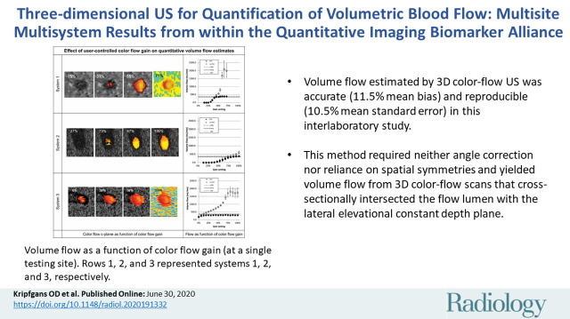
Three-dimensional US for Quantification of Volumetric Blood Flow: Multisite Multisystem Results from within the Quantitative Imaging Biomarkers Alliance

Abstract

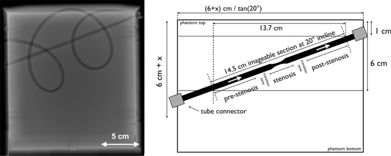
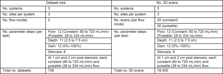
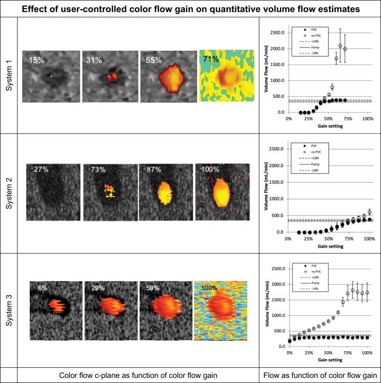
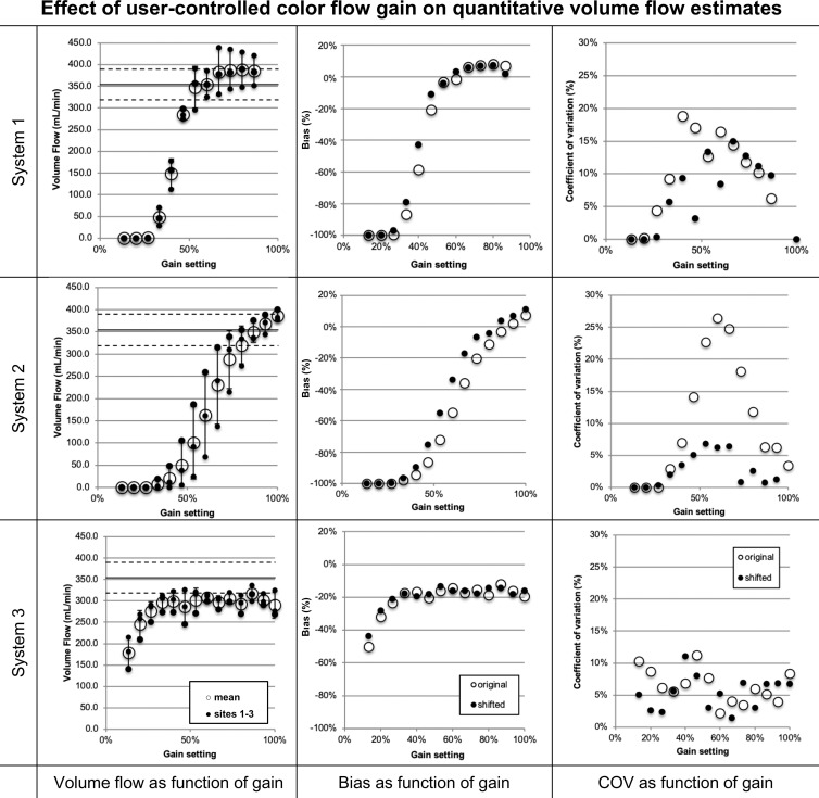
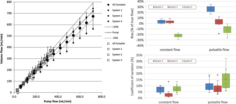
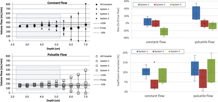
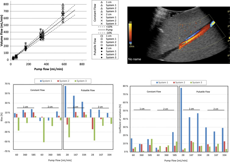
Background Quantitative blood flow (QBF) measurements that use pulsed-wave US rely on difficult-to-meet conditions. Imaging biomarkers need to be quantitative and user and machine independent. Surrogate markers (eg, resistive index) fail to quantify actual volumetric flow. Standardization is possible, but relies on collaboration between users, manufacturers, and the U.S. Food and Drug Administration. Purpose To evaluate a Quantitative Imaging Biomarkers Alliance-supported, user- and machine-independent US method for quantitatively measuring QBF. Materials and Methods In this prospective study (March 2017 to March 2019), three different clinical US scanners were used to benchmark QBF in a calibrated flow phantom at three different laboratories each. Testing conditions involved changes in flow rate (1-12 mL/sec), imaging depth (2.5-7 cm), color flow gain (0%-100%), and flow past a stenosis. Each condition was performed under constant and pulsatile flow at 60 beats per minute, thus yielding eight distinct testing conditions. QBF was computed from three-dimensional color flow velocity, power, and scan geometry by using Gauss theorem. Statistical analysis was performed between systems and between laboratories. Systems and laboratories were anonymized when reporting results. Results For systems 1, 2, and 3, flow rate for constant and pulsatile flow was measured, respectively, with biases of 3.5% and 24.9%, 3.0% and 2.1%, and -22.1% and -10.9%. Coefficients of variation were 6.9% and 7.7%, 3.3% and 8.2%, and 9.6% and 17.3%, respectively. For changes in imaging depth, biases were 3.7% and 27.2%, -2.0% and -0.9%, and -22.8% and -5.9%, respectively. Respective coefficients of variation were 10.0% and 9.2%, 4.6% and 6.9%, and 10.1% and 11.6%. For changes in color flow gain, biases after filling the lumen with color pixels were 6.3% and 18.5%, 8.5% and 9.0%, and 16.6% and 6.2%, respectively. Respective coefficients of variation were 10.8% and 4.3%, 7.3% and 6.7%, and 6.7% and 5.3%. Poststenotic flow biases were 1.8% and 31.2%, 5.7% and -3.1%, and -18.3% and -18.2%, respectively. Conclusion Interlaboratory bias and variation of US-derived quantitative blood flow indicated its potential to become a clinical biomarker for the blood supply to end organs. © RSNA, 2020 Online supplemental material is available for this article. See also the editorial by Forsberg in this issue.

Graphical abstract

Figure 1:

Flow phantom description. Radiograph (left side) shows a linear tube section angled at a 20° incline from left to right. This linear section included a 40% stenosis (ie, a 5- to 3-mm diameter reduction plus subsequent expansion back to 5 mm) over a 3-cm tube length. There is also a curved tubing section that forms two loops. These are intended to be anatomically curved and possess diameter fluctuations with a mean of 5 mm. Schematic (right side) shows the position of stenotic tubing section. Stenotic section and transition zone are not to scale.

Figure 2:

Structure of the multisite multisystem study, with three systems at three different sites per system. The study at each site included four tests (flow, depth, gain, and stenosis) taken under constant and pulsatile flow. This resulted in a total of 738 datasets consisting of 18 450 image volumes. 3D = three-dimensional.

Figure 3:

Volume flow as a function of color flow gain (at a single testing site). For each row the color flow c-plane and the computed volume flow are shown as a function of color flow gain. The c-plane is shown for four representative gain levels, whereas the computed volume flow is shown for 12–17 steps across the available gain settings. Flow was computed with (solid circles on the graphs) and without (hollow circles on the graphs) partial volume correction. Partial volume correction accounts for pixels that are only partially inside the lumen. Therefore, high gain (ie, blooming) does not result in overestimation of flow. Systems 1 and 2 converge to true flow after the lumen is filled with color pixel. System 3 is nearly constant regarding gain and underestimates the flow by approximately 17%. Shown are mean flow estimated from 20 volumes, and the error bars show standard deviation.

Figure 4:

Volume flow as a function of color flow gain. Shown for each row are (left) volume flow (small ●) for systems 1, 2, and 3, respectively, and the mean flow (large ○) and (middle and right) mean bias and coefficient of variation of mean flow between sites (large ○), respectively. Possible differences in system sensitivity between systems 1, 2, and 3 were compensated by allowing a gain offset between sites. The results are shown (small ●). System 2 shows a decrease of coefficients of variation from a maximum of greater than 25% before compensation to 7% after compensation (P = .002). Systems 1 and 3 show no appreciable change. COV = coefficient of variation.

Figure 5:

Computed volume flow as a function of pump flow rate shows volume flow versus pump flow rate (left side), bias in percent of true flow (top right side), and coefficient of variation (lower right side). Data shown are from three systems (blue, red, green) averaged across three sites each at two conditions (constant flow and pulsatile flow). The identity of the systems is hidden by using uniform plot symbols. Constant flow (left) is plotted (●). Mean across systems 1, 2, and 3 is shown (large ●), which are also shown (small ●). Pulsatile flow is plotted (□). The mean (large □) across systems 1, 2, and 3 is shown, and their means are also shown (small □). Box and whisker plots of bias and coefficient of variation for all systems (right side) are shown and split into constant and pulsatile flow. Box plots are shown with error bars (standard deviation), mean (x), median (horizontal line in each box), and 25th–75th percentile range for each system and flow condition. The mean biases (top right) for systems 1, 2, and 3 are, respectively, 3.5%, 3.0%, and −22.1% for constant flow, and 24.9%, 2.1%, and –10.9% for pulsatile flow. Coefficients of variation (bottom right) as box plots for the same data are, respectively, 6.9%, 3.3%, and 9.6% for constant flow and 7.7%, 8.2%, and 17.3% for pulsatile flow.

Figure 6:

Computed volume flow as a function of c-plane (lateral elevational plane of equal distance from the transducer) depth. The left side shows volume flow versus c-plane depth for constant and pulsatile flow in top and bottom panel, respectively. The right side shows box and whisker plots that show bias for each system averaged across sites in percent of true flow within the blue shaded range in the left-side panel. Coefficient of variation is shown (lower right side) for the same blue shaded range of the left-side panel. Data shown are composed of three systems at two conditions, constant flow and pulsatile flow. Constant flow is plotted (upper left side; ●). The mean across systems 1, 2, and 3 is shown (large ●), and each system mean is shown (small ●). The identity of the systems is hidden by using uniform plot symbols. Pulsatile flow is plotted (lower left; □). The mean across systems 1, 2, and 3 is shown (large □), and each system mean is shown (small □). Box plots of bias (top right) and coefficient of variation (bottom right) for all systems are split into constant and pulsatile flow. Box plots are shown with error bars (standard deviation), mean (x), median (horizontal line), and 25th–75th percentile range for each system and flow condition. The mean biases for systems 1, 2, and 3 are, respectively, 3.7%, −2.0%, and −22.8% for constant flow and 27.2%, −0.9%, and −5.9% for pulsatile flow. The mean coefficients of variation are, respectively, 10.0%, 4.6%, and 10.1% for constant flow and 9.2%, 6.9%, and 11.6% for pulsatile flow.

Figure 7:

Volume flow computation of flow distal (downstream) to a 40% stenosis. Computed flow at c-planes (ie, the lateral elevational plane of equal distance from the transducer) located 1 and 2 cm past the stenosis at constant and pulsatile flow conditions. Top left graph shows computed volume flow as a function of pump flow. Constant flow is shown at 1 cm (∆) and 2 cm (×) distal (ie, downstream) to the stenosis and pulsatile flow at 1 cm (□) and 2 cm (●) distal (downstream) to the stenosis, respectively. For constant flow, bias and coefficient of variation are almost all less than 20%. Figure 2 shows analysis of these results. Example screenshot (top right) is shown for poststenotic flow. Bias at 1 and 2 cm poststenosis (bottom left) is shown and averaged between three sites. Coefficient of variation at 1 and 2 cm poststenosis (bottom right) is shown and averaged between three sites.

References

-
- Shung KK. Diagnostic ultrasound: imaging and blood flow measurements. 2nd ed. Boca Raton, Fla: CRC, 2015.
- Gill RW, Kossoff G, Warren PS, Garrett WJ. Umbilical venous flow in normal and complicated pregnancy. Ultrasound Med Biol 1984;10(3):349–363. - PubMed
- Gill RW. Measurement of blood flow by ultrasound: accuracy and sources of error. Ultrasound Med Biol 1985;11(4):625–641. - PubMed
- Holland CK, Clancy MJ, Taylor KJ, Alderman JL, Purushothaman K, McCauley TR. Volumetric flow estimation in vivo and in vitro using pulsed-Doppler ultrasound. Ultrasound Med Biol 1996;22(5):591–603. - PubMed
Publication types
MeSH terms
Substances
Grants and funding
LinkOut - more resources
Full Text Sources
Miscellaneous