Epidemiological analyses of African swine fever in the European Union (November 2017 until November 2018)

Abstract

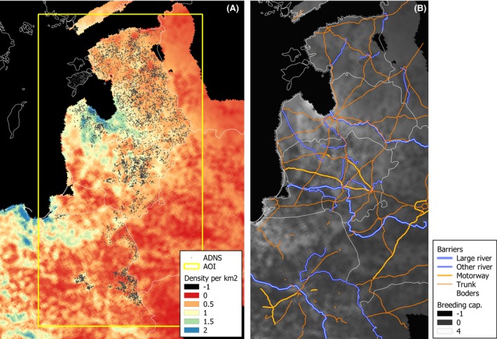
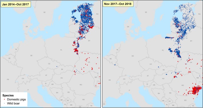
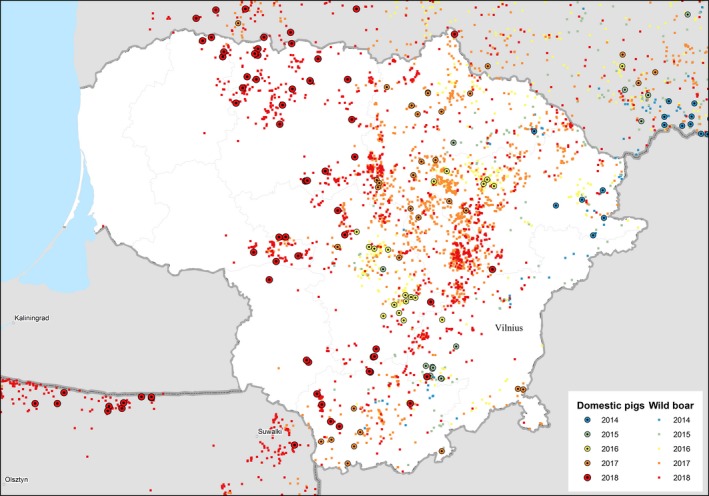
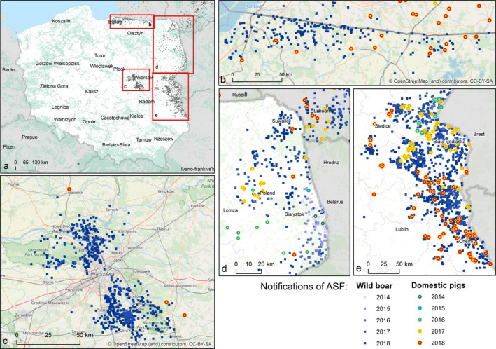
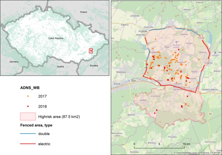
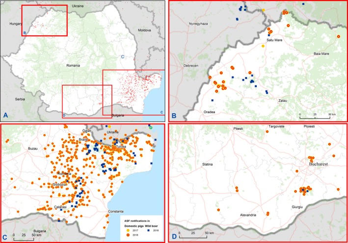
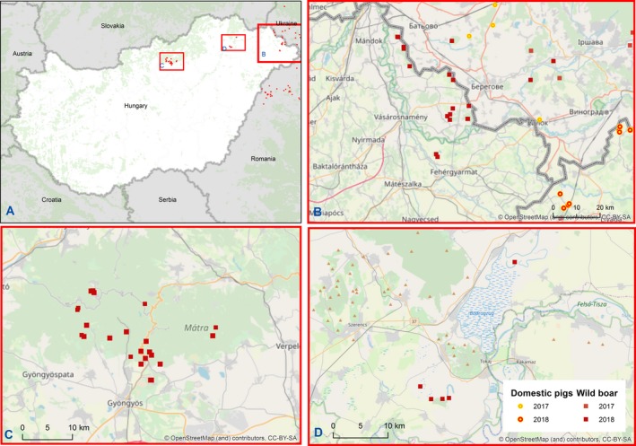
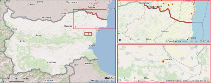
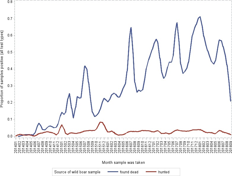
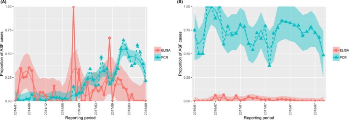
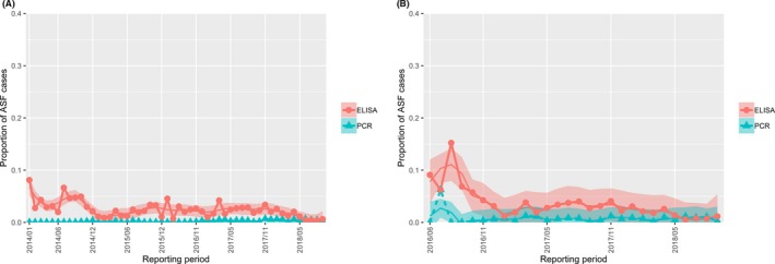
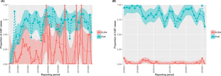
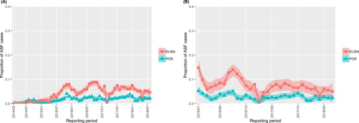
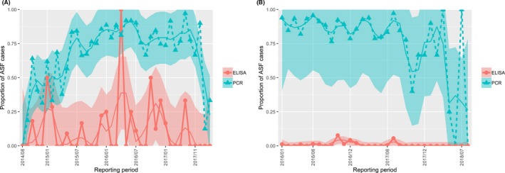
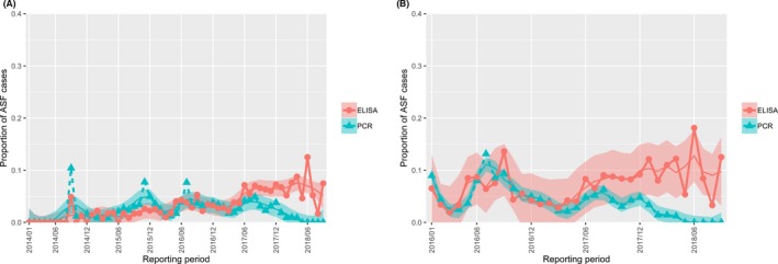
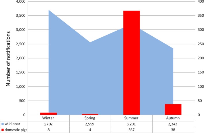
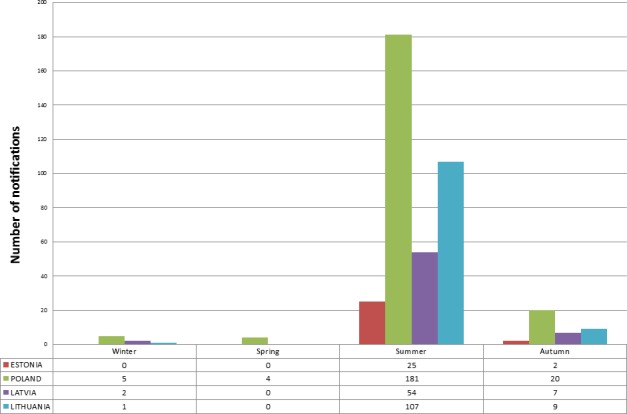
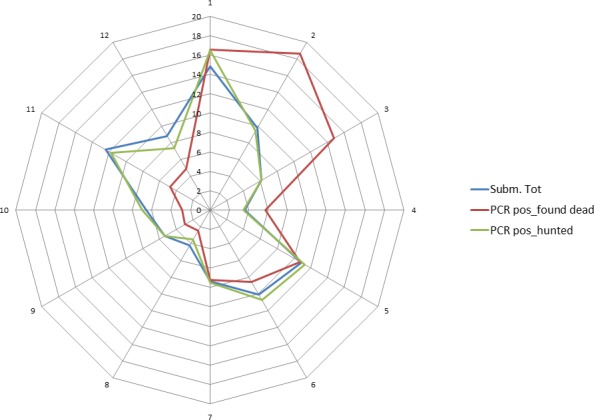
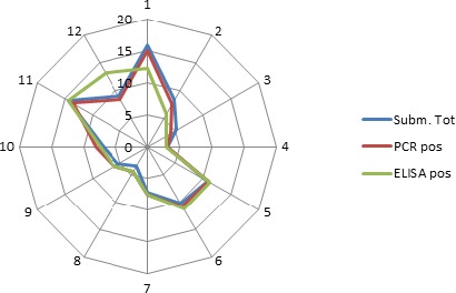
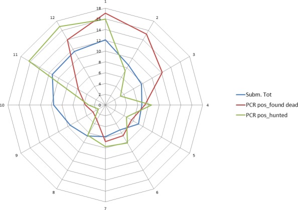
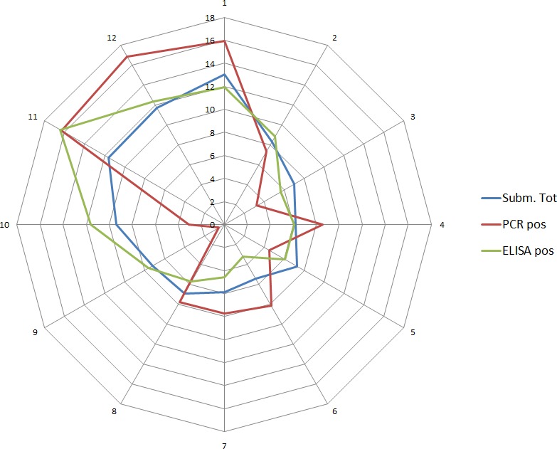
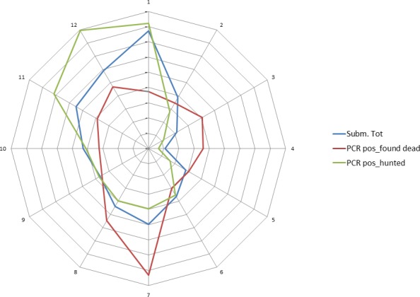
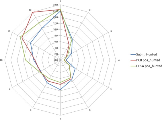
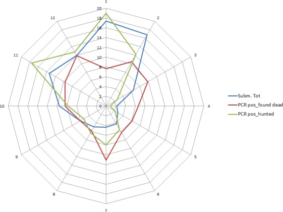
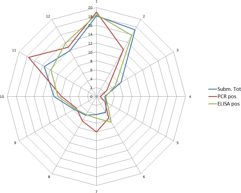
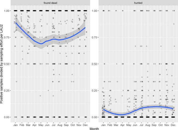
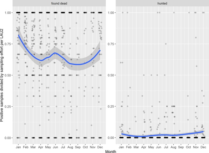
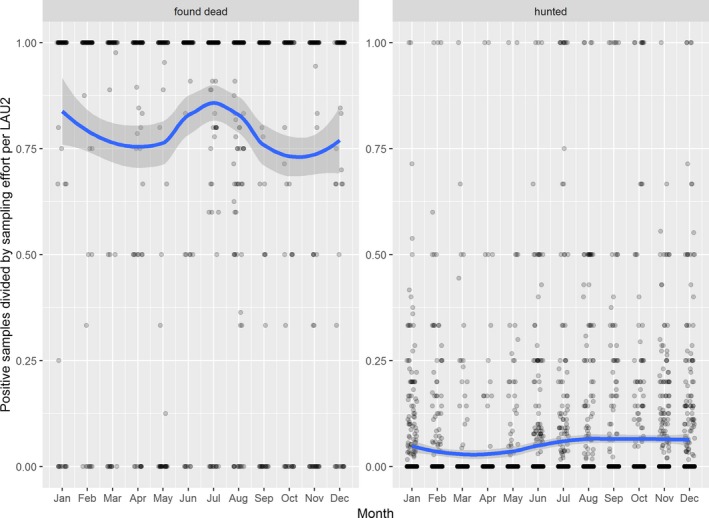
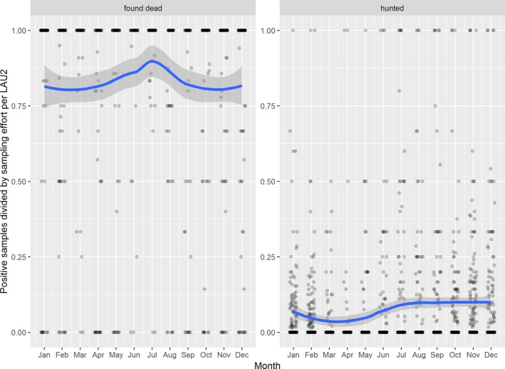
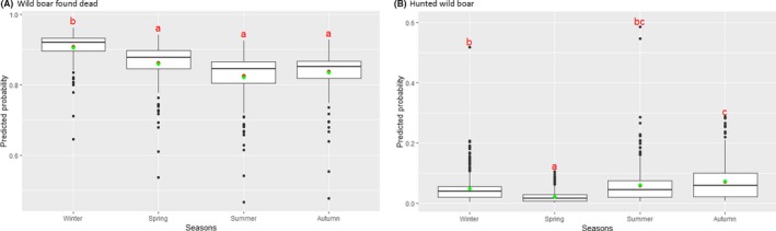
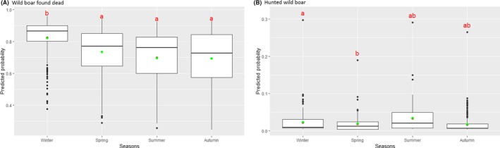
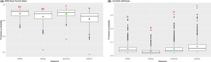
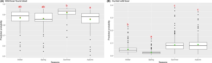
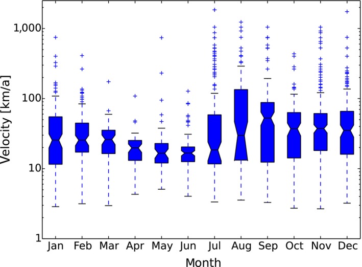
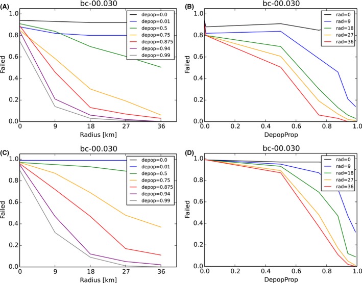
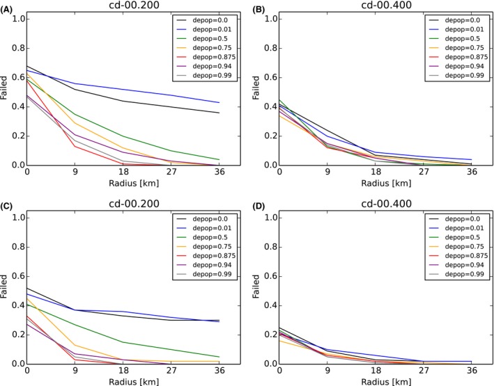
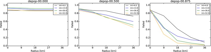
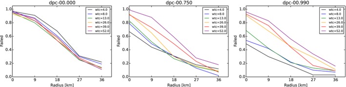
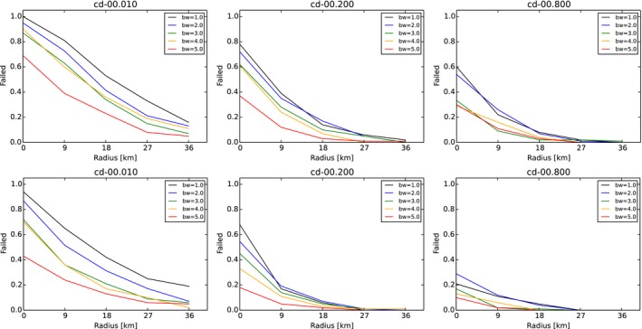
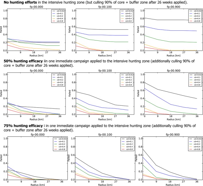
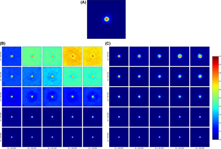
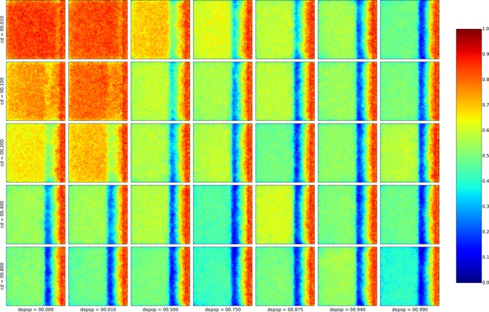
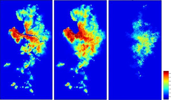
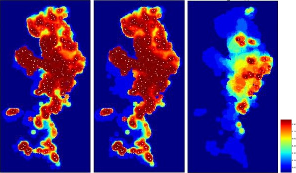
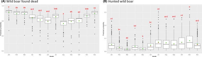
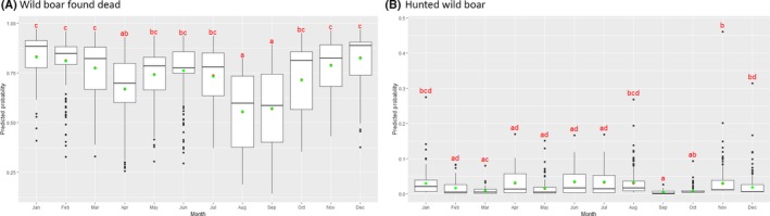
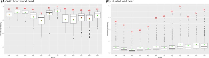
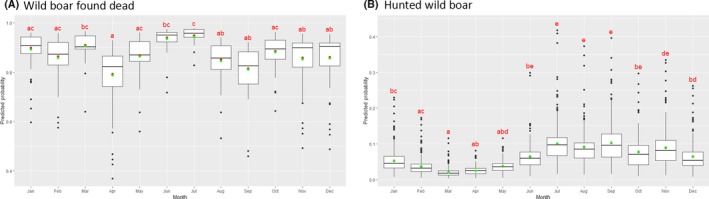
This update on the African swine fever (ASF) outbreaks in the EU demonstrated that out of all tested wild boar found dead, the proportion of positive samples peaked in winter and summer. For domestic pigs only, a summer peak was evident. Despite the existence of several plausible factors that could result in the observed seasonality, there is no evidence to prove causality. Wild boar density was the most influential risk factor for the occurrence of ASF in wild boar. In the vast majority of introductions in domestic pig holdings, direct contact with infected domestic pigs or wild boar was excluded as the route of introduction. The implementation of emergency measures in the wild boar management zones following a focal ASF introduction was evaluated. As a sole control strategy, intensive hunting around the buffer area might not always be sufficient to eradicate ASF. However, the probability of eradication success is increased after adding quick and safe carcass removal. A wider buffer area leads to a higher success probability; however it implies a larger intensive hunting area and the need for more animals to be hunted. If carcass removal and intensive hunting are effectively implemented, fencing is more useful for delineating zones, rather than adding substantially to control efficacy. However, segments of fencing will be particularly useful in those areas where carcass removal or intensive hunting is difficult to implement. It was not possible to demonstrate an effect of natural barriers on ASF spread. Human-mediated translocation may override any effect of natural barriers. Recommendations for ASF control in four different epidemiological scenarios are presented.

Keywords: African swine fever; domestic pigs; epidemiology; management; prevention; risk factor; seasonality; wild boar.

Figure 1

Different wild boar management zones considered in the model

Figure 2

The model realisation of the management scenarios of the focal approach The inner circle (core zone) encircles the detected carcasses (visualised here only live infected animals). Moreover, the model assigns arbitrary number of additional ring‐like zones around the core zone to represent alternative spatial designs and temporal management activity plans. Left: at the moment of implementation of the zones. Right: after eradication of ASF using different culling and hunting scenarios in different zones.

Figure 3

Outcome of the zoning submodel shown by one arbitrary run applying random carcass detection during 4 weeks before delineation of the core zone Red: core zone; yellow: buffer zone; blue: intensive hunting zone.

Figure 4

Habitat model of wild boar and physical barriers for the Baltic countries Left: Carrying capacity values (expressed in density per km²) according to the distribution model proposed by Pittiglio et al. (2018). Right: The carrying capacity overlaid with barriers. Sources: see Lange et al., 2018.

Figure 5

Notifications to the ADNS. Left: notifications from January 2014 to October 2017. Right: notifications from November 2017 to October 2018

Figure 6

ASF outbreaks and cases in domestic pigs and wild boar, respectively, reported to the ADNS in Lithuania (2014–2018) WB = wild boar; ADNS = Animal Disease Notification System.

Figure 7

ASF outbreaks and cases in domestic pigs and wild boar, respectively, reported to the ADNS in Poland

Figure 8

ASF outbreaks and cases in domestic pigs and wild boar, respectively, reported to the ADNS in Latvia

Figure 9

Expansion of the ASF‐infected area in Estonia from September 2014 until December 2016

Figure 10

Occurrence of ASF in domestic pig herds in Estonia from June 2015 to September 2017

Figure 11

ASF outbreaks and cases in domestic pigs and wild boar, respectively, reported to the ADNS in Estonia

Figure 12

ASF cases in wild boar reported to the ADNS in the Czech Republic

Figure 13

ASF outbreaks and cases in domestic pigs and wild boar, respectively, reported to the ADNS in Romania

Figure 14

ASF cases in wild boar reported to the ADNS in Hungary (A); cases in Szabolcs‐Szatmár‐Bereg county (B); Heves county (C); and in Borsod‐Abaúj‐Zemplén county (D)

Figure 15

ASF outbreak domestic pigs reported to the ADNS in Bulgaria

Figure 16

Sixteen ASF cases in wild boar reported to the ADNS in Belgium

Figure 17

Proportion of positive sample over tested samples (PCR and AB‐ELISA) in hunted wild boar and wild boar found dead in the Baltic Countries and Poland since the first introduction

Figure 18

Proportion of ASF‐positive samples over tested samples from all wild boars found dead in the sampled areas of Lithuania (A) and from the affected areas only (B)

Figure 19

Proportion of ASF‐positive samples over tested samples from all hunted wild boar in the sampled areas of Lithuania (A) and from the affected areas only (B)

Figure 20

Proportion of ASF‐positive samples over tested samples from all wild boars found dead in the sampled areas of Poland (A) and from the affected areas only (B)

Figure 21

Proportion of ASF‐positive samples over tested samples from all hunted wild boars in the sampled areas of Poland (A) and from the affected areas only (B)

Figure 22

Proportion of ASF‐positive samples over tested samples from all wild boars found dead in the sampled areas of Latvia (A) and from the affected areas only (B)

Figure 23

Proportion of ASF‐positive samples over tested samples from all hunted wild boars in the sampled areas of Latvia (A) and from the affected areas only (B)

Figure 24

Proportion of ASF‐positive samples over tested samples from all wild boars found dead in the sampled areas of Estonia (A) and from the affected areas only (B)

Figure 25

Proportion of ASF‐positive samples over tested samples from all hunted wild boars in the sampled areas of Estonia (A) and from the affected areas only (B)

Figure 26

Seasonal distribution of ADNS notifications in wild boar and pigs from the Baltic countries and Poland from 2014–2018

Figure 27

Seasonal distribution of ADNS notifications in pigs from the Baltic countries and Poland from 2014–2018

Figure 28

Total numbers of samples submitted for testing (blue) and proportions of PCR‐positive samples from wild boar found dead (red) and hunted wild boar (green) in Lithuania

Figure 29

Total numbers of samples submitted for testing (blue) and proportions of PCR‐positive (red) and ELISA‐positive samples (green) from hunted wild boar in Lithuania

Figure 30

Total numbers of samples submitted for testing (blue) and proportions of PCR‐positive samples from wild boar found dead (red) and hunted wild boar (green) in Poland

Figure 31

Total numbers of samples submitted for testing (blue) and proportions of PCR‐positive (red) and ELISA‐positive samples (green) from hunted wild boar in Poland

Figure 32

Total numbers of samples submitted for testing (blue) and proportions of PCR‐positive samples from wild boar found dead (red) and hunted wild boar (green) in Latvia

Figure 33

Total numbers of samples submitted for testing (blue) and proportions of PCR‐positive (red) and ELISA‐positive samples (green) from hunted wild boar in Latvia

Figure 34

Total numbers of samples submitted for testing (blue) and proportions of PCR‐positive samples from wild boar found dead (red) and hunted wild boar (green) in Estonia

Figure 35

Total numbers of samples submitted for testing (blue) and proportions of PCR‐positive (red) and ELISA‐positive samples (green) from hunted wild boar in Estonia

Figure 36

Lithuania (data available from 2016 to August 2018)

Figure 37

Poland (data available from 2014 to August 2018)

Figure 38

Latvia (data available from 2014 to August 2018)

Figure 39

Estonia (data from available 2014 to August 2018)

Figure 40

Comparison of seasonal ASF incidence using a generalised linear mixed model and Tukey pairwise comparison for Lithuania

Figure 41

Comparison of seasonal ASF incidence using a generalised linear mixed model and Tukey pairwise comparison for Poland

Figure 42

Comparison of seasonal ASF incidence using a generalised linear mixed model and Tukey pairwise comparison for Latvia

Figure 43

Comparison of seasonal ASF incidence using a generalised linear mixed model and Tukey pairwise comparison for Estonia

Figure 44

Seasonal variation of local expansive spread or local velocity (10 × 10 km) of infection measured by notifications (source: ADNS). Human‐mediated longer distance translocations are disentangled from the wild boar‐related spatial spread

Figure 45

Aggressive interactions among wild boar, a likely means of ASFV transmission, can take place at local attractive resources such as feeding sites, or during the mating season

Figure 46

Network representation of ASF detections in Estonia, with outbreaks paired based on closest time and distance

Figure 47

Statistically significant hot spots using the Getis‐Ord Gi* statistic (taking into account the number of cases)

Figure 48

Human‐made translocations

Figure 49

Temporal estimated probabilities for each LAU2 region showing the probability of observing African swine fever cases in Estonia for each year since the introduction

Figure 50

Spatial predictions for each LAU2 region in Estonia of probabilities of observing African swine fever for each year since the introduction

Figure 51

Example and variability of the model output. The probability is shown that the implemented measures fail to prevent ASF spread out of the intensive hunting area as function to its width. Thirty lines show variability by representing the same output measure produced of the standard approach, i.e. 100 simulation runs (total 3,000 simulation runs). Every run applies identical parameters

Figure 52

Simulation output on effect size of alternative hunting efforts at different width of the intensive hunting zone (without carcass removal and without fence around core zone) or percentage of wild boar population hunted in the intensive hunting zone Top: carcass contacts only after 2 weeks (in line with Probst et al., 2017). Bottom: carcass contacts possible right after death. The same data are summarised as a function of hunting zone width (left) and annual depopulation efficacy (right). In the intensive hunting zone annual depopulation efficacy is set in per cent (coloured line graphs) and achieved every year with two campaigns. Each campaign was completed within 4 weeks. The protocol is repeated annually until the end of the simulations. In the core + buffer zones one campaign is performed after a half‐year waiting period, applying 90% reduction of animals still present.

Figure 53

Simulation output on the effect of alternative carcass removal rate (carcass removal = cd, see diagram title) and width of as well as efficiency in the intensive hunting zone (x‐axis) The core zone is delineated using either random carcass detections within 4 weeks (top two diagrams) or perfect knowledge on carcass distribution prior to zoning (bottom two diagrams; remember only knowledge of carcass was perfect not removal, latter as in top row). Independent of the annual depopulation efficacy in (coloured lines) or width of the intensive hunting zone (x‐axis), logically, only carcass removal rate in the core + buffer zone can determine the failure rate out of the core + buffer zone (equally coloured line graphs at x‐axis zero value compared between left and right at CD = 20% and CD = 40% carcasses removed). As before, increased hunting effort in the intensive hunting zone further improves success chance (coloured lines per diagram). The hunting target was achieved every year with two campaigns. Each campaign was completed within 4 weeks. The protocol is repeated annually until the end of the simulations. In the core + buffer zones one campaign is performed after a half‐year waiting period, applying 90% culling of animals still there.

Figure 54

Simulation output on effect of alternative scheduling of hunting campaigns (i.e. varying the interval between hunting campaigns) while guaranteeing equal overall annual hunting efficacy (without carcass removal) The depopulation efficacy over the year is 0%; 50%; 88% (see diagram title).The parameter interval (int) refers to the interval in weeks between the performance of the consecutive hunting campaigns in the intensive hunting zone; int = 52 means one 4‐week campaign per year with greatest efforts; int = 4 means 13 four‐week campaigns per year i.e. hunting every week with lesser efforts. Effort per campaign is adjusted to achieve in summary the annual efficacy of depopulation per cent. NB: The culling measures in the core + buffer zone did not alter over all simulations and were set at 90% as after 26 weeks waiting time

Figure 55

Culling efficacy in the core + buffer zone in one campaign for different waiting times between the start of all applied measures and the start of culling in the core + buffer zone Failure rate is given for different waiting times (waiting times = wtc; coloured lines) between start of measures and culling in the core + buffer zone. Three scenarios for the culling efficacy (see dpc; diagram title) of 0% (left), 75% (middle) and 99 % right are shown.

Figure 56

The effect of the width of the buffer zone on the final success assuming alternative carcass removal rates The width of the buffer zone (bw) is represented by the coloured lines: black 1; blue 2; green 3; yellow 4; and red 5 times the wild boar group home range). The standard parameter used in scenarios above refers to buffer width (bw) = 3. Carcass detections and removal rate (cd; diagram title) is either 10% (left), 20% (middle); 80% right. Independently, the core zone is delineated based on random carcass detections during 4 weeks after ASF confirmation (top row) or perfect knowledge on carcass distribution (bottom row). The hunting efficiency in the intensive hunting zone is set to 75% distributed over two campaigns per year. Waiting time until culling of the core + buffer zone was 26 weeks and achieved by one campaign with 90% efficacy.

Figure 57

Example of simulation analysis showing true infection status of the wild boar groups at the moment of zoning (4 weeks following first notification) based on perfect knowledge about distribution of carcasses from animals that died from ASFV infection The 100% wild boar‐proven fence was built around the core zone (white area) – while already newly infected animals have reached the buffer zone (light grey area). As a consequence, simulations assuming a 100% wild boar‐proven fence can also fail to stop the spread of ASF.

Figure 58

Simulation output as failure rate out of 100 repetitions of scenarios. Scenarios differ by different fence permeability, hunting efficacy, carcass detection rate and the width of the intensive hunting zone Row‐wise: Different hunting efficacy (top 0%; 50%; 75% i.e. during the annual 4‐week campaign, with any animal having the chance to be hunted with the given percentage value); Column‐wise: Different permeability of the fence (left 0% i.e. wild boar proof; middle 10%; right 90% nearly absent); Colour of the lines: Different carcass detection rate (black 1%; blue 10%; green 20%; yellow 40%; red 80%); x‐axis: width of the intensive hunting zone (0, 3, 6, 9, 12 times the wild boar group home ranges of 3 km); y‐axis: Proportion of runs failed to be halted, or 1‐success rate of the measure at a given hunting zone width.

Figure 59

Spatial simulation output shown as a heat map of the proportion of 100 repetitions of alternative scenarios Scenarios differed by applied control measures. (A) Enlargement of top‐left in (C) assuming the presence of a wild boar‐proof fence around the core zone, red area approximates the overlaid core zones of 100 runs, yellow, i.e. a much lower proportion, the buffer zones. The surrounding halos reveal the limited spread due to very high hunting efforts in the intensive hunting zone. (B) and (C) Scenario comparison for different levels of hunting i.e. 0% in (B) and 75% in (C). Both (B) and (C) cross‐tabulate column‐wise different permeability of the fence (left 0% wild boar proof; 5%; middle 10%; 50%; right 90% fence nearly absent) vs row‐wise different carcass detection rates (top 1%; 10%; middle 20%; 40%; bottom 80%). Zoning is based on perfect knowledge about infectious carcass distribution at the moment of zoning (results for 10% chance of carcass detection, see Lange et al., 2018).

Figure 60

Spatial simulation output shown as a heat map of the proportion of 100 repetitions of alternative scenarios addressing the large‐scale control of ASF to stop wild boar‐mediated spread into areas at higher risk of ASF introduction by wild boar‐mediated spread Scenarios differed by applied control measures. Column‐wise: different hunting efforts in the intensive hunting zone (left 0%; 1%; 50%; middle 75%; 87%; 94%, right 99%) vs row‐wise different carcass detection rates (top 1%; 10%; middle 20%; 40%; bottom 80%). The more reddish a pixel is coloured the higher the proportion of 100 repetitions for the scenario in which the respective wild boar group became affected.

Figure 61

Probability to receive an ASF infection in wild boar dependent on physical barriers and likely human‐mediated translocations Heat map of 100 repetitions. Higher value (reddish) shows greater probability. Left: Forced simulation assuming impermeable barriers (blocking walls); Middle: Forced simulation (see section 2.2.4) assuming fully permeable barriers; Right: As middle but without forcing from March 2015 onwards. White pixels represent forcing locations based on the excess values in local velocity.

Figure 62

Jaccard similarity map between ADNS and the final outcome of 100 repetitions considering combinations of physical barriers and likely human‐mediated translocations Higher value (reddish) show greater similarity. Left: Forced simulation assuming impermeable barriers (blocking walls); Middle: Forced simulation assuming fully permeable barriers; Right: As middle but without forcing from March 2015 onwards. White pixels represent forcing locations based on the excess values in local velocity.

Figure C.1

Comparison of monthly ASF incidence using a generalised linear mixed model and Tukey pairwise comparison for Lithuania

Figure C.2

Comparison of monthly ASF incidence using a generalised linear mixed model and Tukey pairwise comparison for Poland

Figure C.3

Comparison of monthly ASF incidence using a generalised linear mixed model and Tukey pairwise comparison for Latvia

Figure C.4

Comparison of monthly ASF incidence using a generalised linear mixed model and Tukey pairwise comparison for Estonia

References

1. Acevedo P, Vicente J, Höfle U, Cassinello J, Ruiz‐Fons JF and Gortázar C, 2007. Estimation of European wild boar relative abundance and aggregation: a novel method in epidemiological risk assessment. Epidemiology and Infection, 135, 519–527. - PMC - PubMed
1. Albrycht M, Merta D, Bobek J and Ulejczyk S, 2016. The demographic pattern of wild boars (Sus scrofa) inhabiting fragmented forest in north‐eastern Poland. Baltic Forestry, 22, 251–258.
1. Barasona JA, Acevedo P, Diez‐Delgado I, Queiros J, Carrasco‐García R, Gortázar C and Vicente J, 2016. Tuberculosis‐associated death among adult wild boars, Spain, 2009–2014. Emerging Infectious Diseases, 22, 2178–2180. 10.3201/eid2212.160677 - DOI - PMC - PubMed
1. BFSA (Bulgarian Food Safety Agency), 2018. African swine fever control measures in Bulgaria. Presentation at the PAFF meeting, 12–13 July 2018, Brussels. Available online: https://ec.europa.eu/food/sites/food/files/animals/docs/reg-com_ahw_2018... [Accessed: 31 October 2018].
1. Boadella M, Vicente J, Ruiz‐Fons F, de la Fuente J and Gortázar C, 2012. Effects of culling Eurasian wild boar on the prevalence of Mycobacterium bovis and Aujeszky's disease virus. Preventive Veterinary Medicine, 107, 214–221. 10.1016/j.prevetmed.2012.06.001 - DOI - PubMed
LinkOut - more resources