Spinning disk-remote focusing microscopy

Abstract

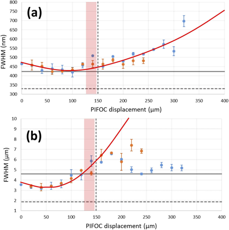
Fast confocal imaging was achieved by combining remote focusing with differential spinning disk optical sectioning to rapidly acquire images of live samples at cellular resolution. Axial and lateral full width half maxima less than 5 µm and 490 nm respectively are demonstrated over 130 µm axial range with a 256 × 128 µm field of view. A water-index calibration slide was used to achieve an alignment that minimises image volume distortion. Application to live biological samples was demonstrated by acquiring image volumes over a 24 µm axial range at 1 volume/s, allowing for the detection of calcium-based neuronal activity in Platynereis dumerilii larvae.

Fig. 1.

Simplified optical scheme of the combined SD-RF setup: Structured excitation light from the spinning disk (SD) is imaged through the remote focusing unit and onto the sample. Sample fluorescence is collected by O1 (40X 0.8NA, water dipping) and the magnified image is demagnified by the refocusing lens, O2 (40X 0.95 NA air). A third reimaging objective O3, identical to O2, relays an image of the sample plane, back onto the spinning disk (SD). In-focus fluorescence passes through the upper path onto one half of the sCMOS camera (CAM), with the out of focus component passing through the lower path onto the second half of the camera detector. On-the-fly processing of the two images then returns a confocal image of the sample. By scanning and de-scanning in Z, the position of O3 determines the axial location of plane of interest in the sample (see main text). FM = fold mirror, DM = dischroic mirror. Tube lenses L1 (f = 180 mm) and L2 (f = 140 mm).

Fig. 2.

(A) A fluorescent calibration pattern written into low index polymer (n = 1.34) showing first layer in a 3D array of features. (B) Axial intensity profile (blue line) within an ROI encircling a single fluorescent feature in the array. The average axial separation of 8.76 µm between layers was measured by fitting a Gaussian (red dashed line) to the axial intensity profile across each layer and calculating the separation of the Gaussian peaks.

Fig. 3.

Variation in lateral magnification as a function of refocusing depth for the SD-RF system. The change in magnification was < 3% over a 400 µm range. Data (blue dots) and line of best fit (red line) are shown. Dashed black lines indicate a magnification of 51.1 at the focal plane of the imaging objective.

Fig. 4.

Measured lateral (a) and axial (b) resolutions (FWHM) for RF-only (orange dots) and SD-RF (blue dots) imaging configurations, together with trend line (solid red line). Also shown are the imaging objective focal plane (vertical dashed black lines), theoretical resolution limits (dashed grey lines), resolution values measured at the side-port (solid grey lines) and the axial range over which live image data was taken (pink bars).

Fig. 5.

(a) Timing diagram for the SD-RF during acquisition. (b). Sketch showing the locations of the acquired frames and the sample relative to the Z values used by the PIFOC. Anterior neural plexus highlighted in yellow. Image of Platynereis adapted from Fig. 1(F), [19].

Fig. 6.

Four of the five optical sections taken from the anterior nervous system region of Platynereis dumerilii (anterior view). Sections are axially separated by 6 µm over a 24 µm depth range. 50 ms exposures are captured at a rate of 5 Hz. Scale bar 50 µm.

Fig. 7.

Measuring changes in electrical activity through Ca²⁺ binding to GCaMP. Three regions of interest were defined for each of the four planes. (a) Overlays on the Z = 128 µm plane show the location of the three regions of interest (ROI). Scale bar 50 µm. (b) Traces showing fluorescence changes relative to average fluorescence (ΔF/F) within the colour coded ROI across all time points. Plots are shown in vertically offset for clarity. Overlays indicate values of ΔF/F at each of the time points shown.

Fig. 8.

Multichannel images of fixed Platynereis dumerilii larvae after (a) 2 days post-fertilisation and (b) 3 days post-fertilisation. Labels: (a) blue (DAPI) = nuclei; red (DsRed) = pERK immunostaining, (b) red = THDa immunostaining, green = cilia bands (acetylated tubulin immunostaining). Scale bars (a) 30 µm (b) 50 µm.

Fig. 9.

(a) A test sample used to measure the PSF with and without the presence of a coverslip. A layer of dried beads on a microscope slide is half covered by a coverslip which is held in place by a second plastic slide with circular aperture. The beads can then be imaged with and without a coverslip by a small lateral displacement of the sample. (b) XZ PSF profiles obtained using the test sample in (a), showing negative spherical aberration introduced by the coverslip and the corresponding axial displacement.

References

1. Nadella K. N. S., Roš H., Baragli C., Griffiths V. A., Konstantinou G., Koimtzis T., Evans G. J., Kirkby P. A., Silver R. A., “Random-access scanning microscopy for 3D imaging in awake behaving animals,” Nat. Methods 13(12), 1001–1004 (2016).10.1038/nmeth.4033 - DOI - PMC - PubMed
1. Grewe B. F., Voigt F. F., van ’t Hoff M., Helmchen F., “Fast two-layer two-photon imaging of neuronal cell populations using an electrically tunable lens,” Biomed. Opt. Express 2(7), 2035–2046 (2011).10.1364/BOE.2.002035 - DOI - PMC - PubMed
1. Corbett A. D., Burton R. A. B., Bub G., Salter P. S., Tuohy S., Booth M. J., Wilson T., “Quantifying distortions in two-photon remote focussing microscope images using a volumetric calibration specimen,” Front. Physiol. 5, 384 (2014).10.3389/fphys.2014.00384 - DOI - PMC - PubMed
1. Göbel W., Kampa B. M., Helmchen F., “Imaging cellular network dynamics in three dimensions using fast 3D laser scanning,” Nat. Methods 4(1), 73–79 (2007).10.1038/nmeth989 - DOI - PubMed
1. Botcherby E. J., Juškaitis R., Booth M. J., Wilson T., “An optical technique for remote focusing in microscopy,” Opt. Commun. 281(4), 880–887 (2008).10.1016/j.optcom.2007.10.007 - DOI
LinkOut - more resources