Computation Through Neural Population Dynamics

Abstract

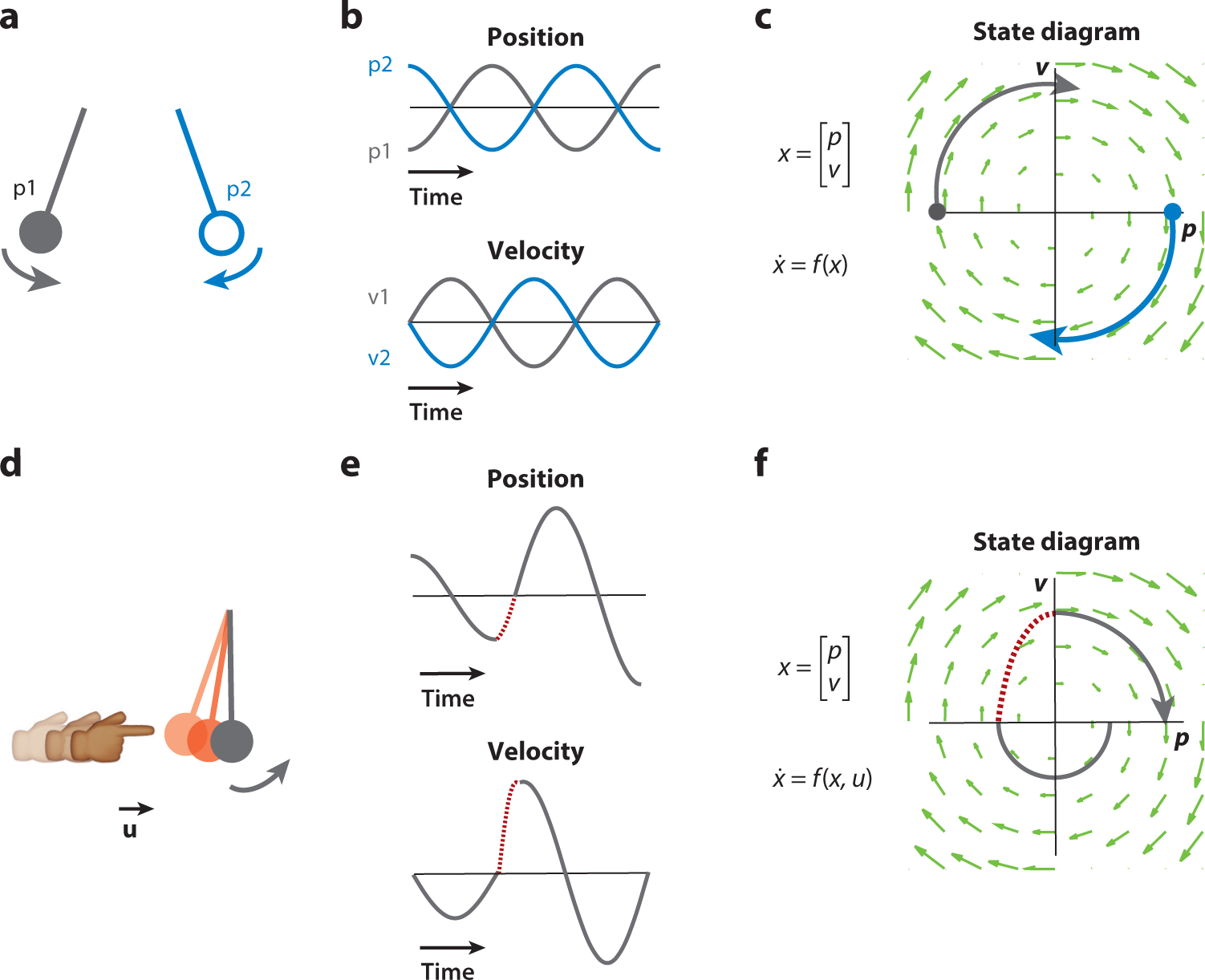
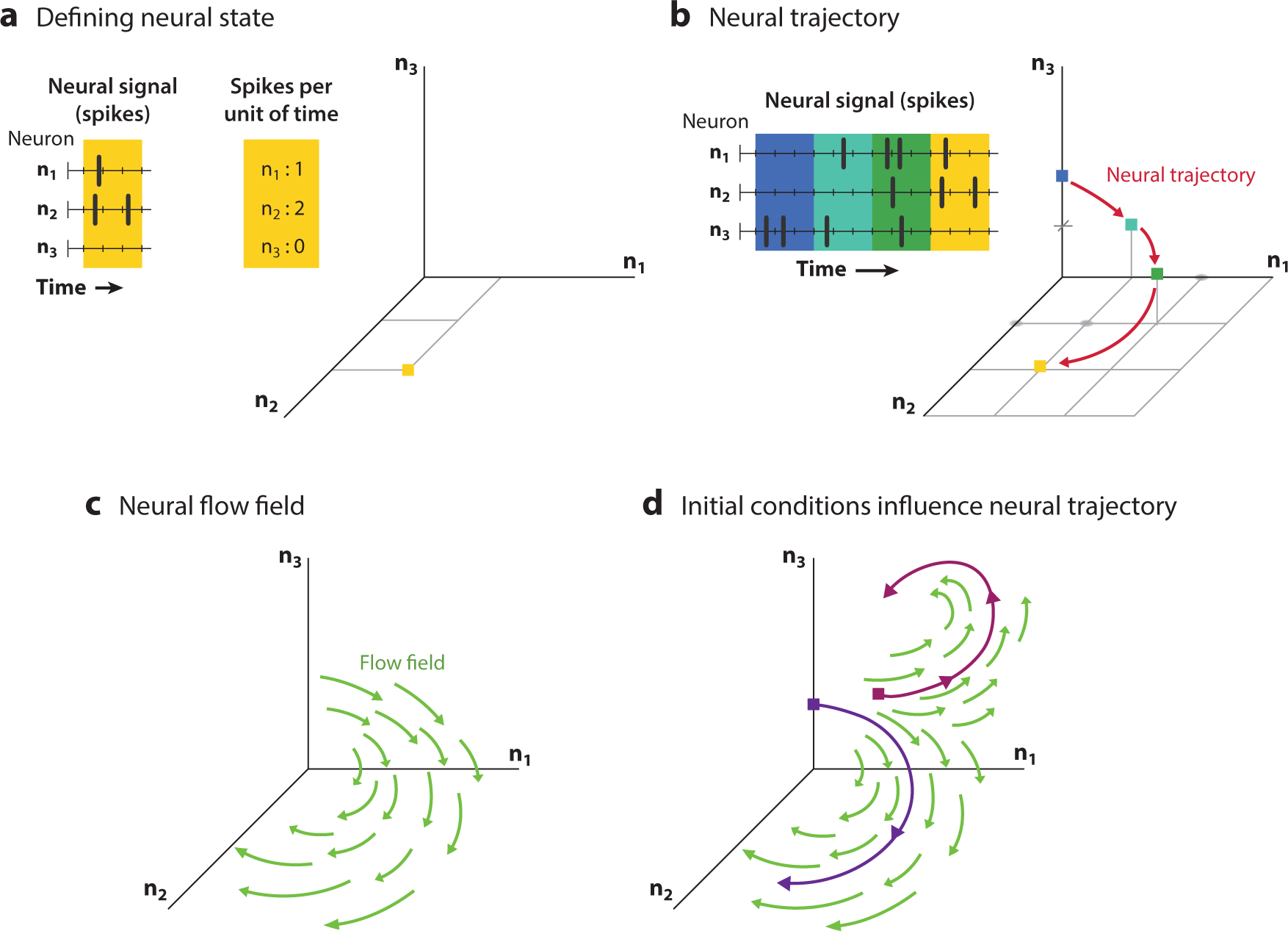
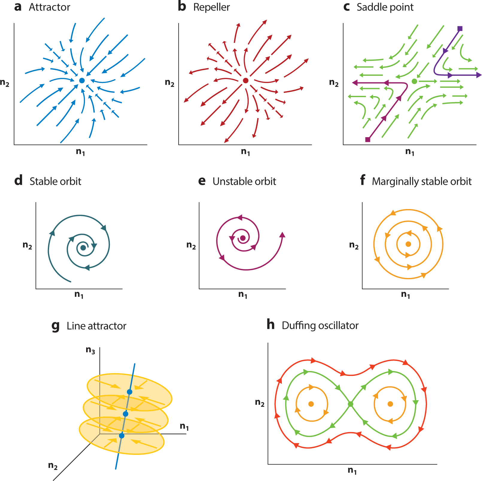
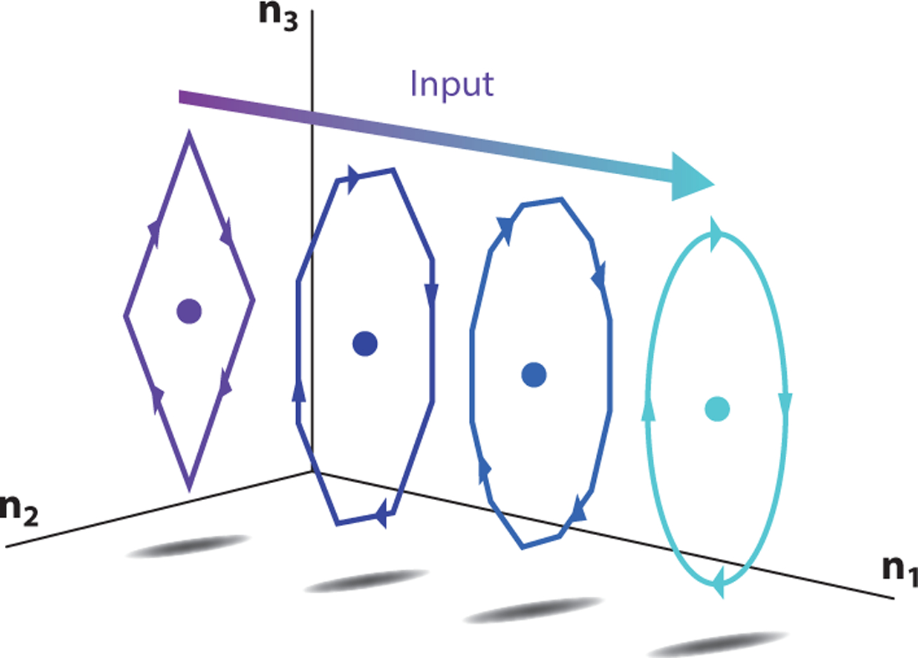
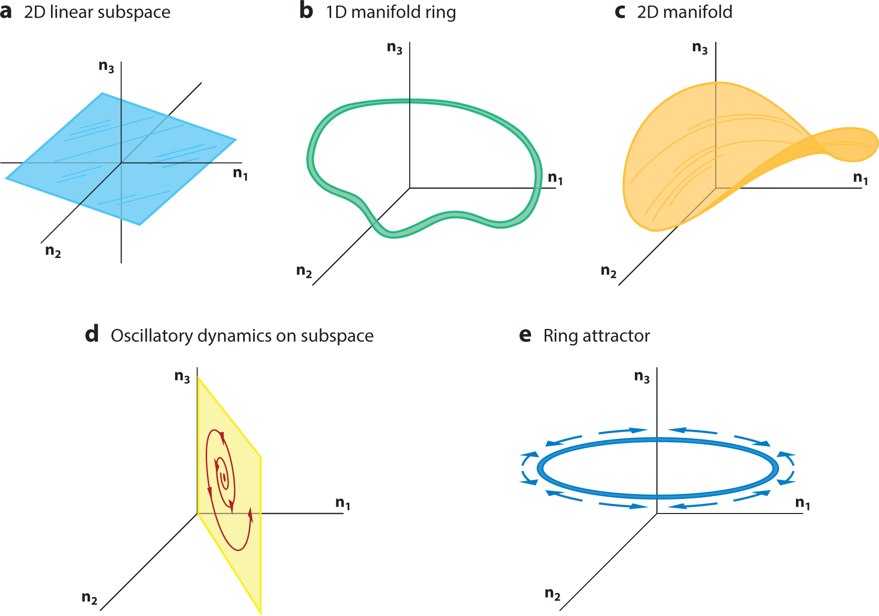
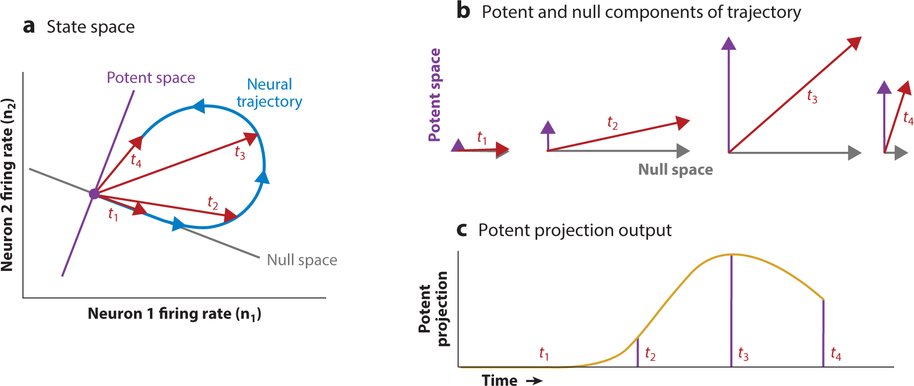
Significant experimental, computational, and theoretical work has identified rich structure within the coordinated activity of interconnected neural populations. An emerging challenge now is to uncover the nature of the associated computations, how they are implemented, and what role they play in driving behavior. We term this computation through neural population dynamics. If successful, this framework will reveal general motifs of neural population activity and quantitatively describe how neural population dynamics implement computations necessary for driving goal-directed behavior. Here, we start with a mathematical primer on dynamical systems theory and analytical tools necessary to apply this perspective to experimental data. Next, we highlight some recent discoveries resulting from successful application of dynamical systems. We focus on studies spanning motor control, timing, decision-making, and working memory. Finally, we briefly discuss promising recent lines of investigation and future directions for the computation through neural population dynamics framework.

Keywords: dynamical systems; neural computation; neural population dynamics; state spaces.

Figure 1

Example dynamics and population state of a frictionless pendulum. (a–c) A pendulum is a 2D dynamical system that has a simple relationship between the changes of the state of the pendulum (1D position and 1D velocity) and its current state. (a) Two example initial conditions are shown, p1 (gray; position is maximally negative and velocity is zero) and p2 (blue; position is maximally positive and velocity is zero). (b) As the pendulum moves through time, its state vector (position, top; velocity, bottom) is updated. (c) These trajectories can also be visualized by plotting one state variable against the other (position against velocity), beginning at the initial condition (circles) and moving along the flow field (green arrows), yielding the state space plot. The flow field shows the dynamical evolution of the pendulum for any set of initial conditions. (d–f) A pendulum with input perturbations. (d) One may perturb the pendulum during its motion, for example, by bumping it with a finger (brief period of the bumps appears in red). (e,f) This leads to a change in the pendulum state through time (red dashed lines) such that both the time series (e) and the state space trajectories (f) no longer follow the autonomous dynamics (as shown in panel e) while the input is active. After the perturbation is finished, the pendulum returns to its autonomous dynamics again (gray lines after red dashed lines). Figure adapted with permission from Pandarinath et al. (2018b).

Figure 2

Neural population state and neural dynamics. (a) Three neurons spike through time (left), and these spikes are binned and counted (center). These spike counts are plotted in a three-dimensional state space (right) representing the three neurons (n₁, n₂, n₃), with a yellow square representing the state of the neural system at that time point. (b) Continued binning of spikes through time (left) leads to a neural population state that progresses in a sequence (blue, cyan, green, yellow), which is plotted in the neural state space plot (right) to yield an intuitive picture of the neural population dynamics. (c) The neural population dynamics can be represented by a flow field (green arrows) that describes how the neural population state evolves through time. (d) Two different neural trajectories (magenta and purple curves) can result from following the neural population dynamics from different initial conditions (magenta and purple squares).

Figure 3

Linear dynamics and linear approximations of nonlinear systems around fixed points. (a–g) Examples of linearized dynamics around fixed points in a nonlinear system, showing fixed points (large dots) and flow fields (arrows). Panels show (a) an attractor, which is stable in all dimensions; (b) a repeller, which is unstable in all dimensions; and (c) a saddle point, which is a fixed point with both stable and unstable dimensions. Fixed points can have oscillatory dynamics that are both (d) stable and (e) unstable. Linear systems that are finely tuned may have marginally stable oscillations, which neither decay nor expand, or (f) exhibit line attractor dynamics, (g) which are stable (do not move) along the line attractor (blue line) but otherwise show stable attracting dynamics to the line attractor (yellow planes and arrows). (h) A nonlinear system such as a Duffing oscillator is well approximated by linear systems at the three fixed points: The two orange points are well approximated by oscillatory linear dynamics, while the green point is a saddle point, whose dynamics are well approximated by linear dynamics that are both stable and unstable. Note the flow fields given by the red line are not well approximated by linearization, highlighting a failure mode of linearization around fixed points in that good approximations tend to be local.

Figure 4

Contextual inputs. A static or slowly varying input can be viewed as contextualizing a nonlinear system such that it produces different dynamics under different values of the contextual input. In this diagram, increasing the value of a static input (from purple for small values to cyan for large values) moves the operating point of the nonlinear system (circles) such that the dynamics smoothly change from a diamond-like oscillation (purple arrows) to a circular oscillation (cyan arrows).

Figure 5

Subspaces and manifolds. (a) Two-dimensional (2D) linear subspace (blue) embedded in a three-dimensional (3D) space. (b) One-dimensional (1D) ring manifold (green) embedded in 3D space. (c) A smooth 2D manifold (orange) embedded in 3D space. (d,e) Dynamics may live in subspaces or on manifolds. (d) A 2D oscillation embedded in a 2D linear subspace, all of which is embedded in 3D space. (e) A ring attractor, which is a 1D manifold of stable fixed points (blue ring) embedded in 3D space. Inputs move the state along the ring attractor (blue arrows; note arrows here indicate the effect of inputs, not flow fields).

Figure 6

Null and potent subspaces. A state space can be divided up into nonoverlapping subspaces, called the potent and null (sub)spaces, where the potent space may be read out by a downstream area, while the null space is not read out. (a) A dynamical trajectory (blue arrows) in state space follows a looping dynamic from the origin back to the origin. While doing so, the trajectory has projections on the null space (gray line) and potent space (purple line). We focus on four points in time, t₁, t₂, t₃, and t₄ (red arrows). (b) The state space trajectory in panel a can be decomposed into its projections onto the potent and null spaces (shown for time points t₁, t₂, t₃, and t₄). (c) The projection of the state space trajectory onto the potent dimension through time (yellow line), highlighting its value at time points t₁, t₂, t₃, and t₄. There is a corresponding time series for the projection onto the null space (not shown), but this is not read out by a downstream area. Examples of this in systems neuroscience can be found in these references (Hennig et al. 2018, Kaufman et al. 2014, Perich et al. 2018, Semedo et al. 2019, Stavisky et al. 2017a).

References

1. Adamantidis A, Arber S, Bains JS, Bamberg E, Bonci A, et al. 2015. Optogenetics: 10 years after ChR2 in neurons—views from the community. Nat. Neurosci 18:1202–12 - PubMed
1. Afshar A, Santhanam G, Yu BM, Ryu SI, Sahani M, Shenoy KV. 2011. Single-trial neural correlates of arm movement preparation. Neuron 71(3):555–64 - PMC - PubMed
1. Ahrens MB, Li JM, Orger MB, Robson DN, Schier AF, et al. 2012. Brain-wide neuronal dynamics during motor adaptation in zebrafish. Nature 485(7399):471–77 - PMC - PubMed
1. Allen WE, Chen MZ, Pichamoorthy N, Tien RH, Pachitariu M, et al. 2019. Thirst regulates motivated behavior through modulation of brainwide neural population dynamics. Science 364(6437):eaav3932 - PMC - PubMed
1. Ames KC, Churchland MM. 2019. Motor cortex signals for each arm are mixed across hemispheres and neurons yet partitioned within the population response. eLife 8:e46159. - PMC - PubMed
Publication types
LinkOut - more resources