Mechanical Heterogeneity in the Bone Microenvironment as Characterized by Atomic Force Microscopy

Abstract

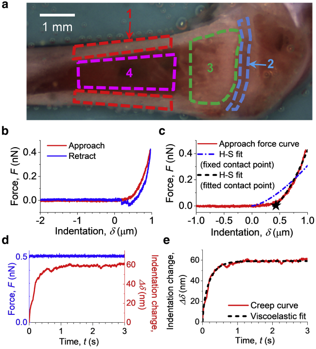
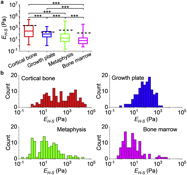
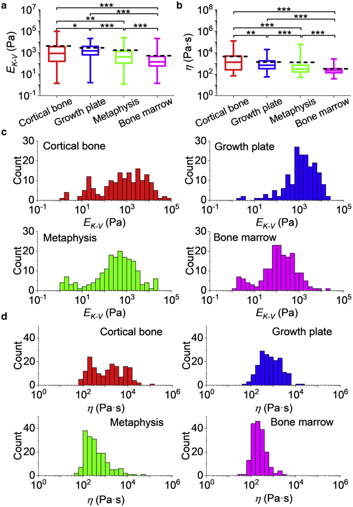
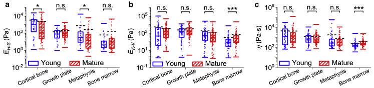
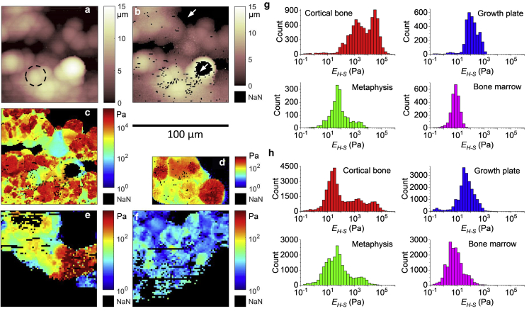
Bones are structurally heterogeneous organs with diverse functions that undergo mechanical stimuli across multiple length scales. Mechanical characterization of the bone microenvironment is important for understanding how bones function in health and disease. Here, we describe the mechanical architecture of cortical bone, the growth plate, metaphysis, and marrow in fresh murine bones, probed using atomic force microscopy in physiological buffer. Both elastic and viscoelastic properties are found to be highly heterogeneous with moduli ranging over three to five orders of magnitude, both within and across regions. All regions include extremely compliant areas, with moduli of a few pascal and viscosities as low as tens of Pa·s. Aging impacts the viscoelasticity of the bone marrow strongly but has a limited effect on the other regions studied. Our approach provides the opportunity to explore the mechanical properties of complex tissues at the length scale relevant to cellular processes and how these impact aging and disease.

Figure 1

Method for measuring the mechanical properties on internal bone surfaces. (a) Bright field image of a prepared bone surface for AFM characterization. Four regions of interest are indicated by colored dashed lines: 1) cortical bone (red), 2) the growth plate (blue), 3) the metaphysis (green), and 4) bone marrow in diaphysis (magenta). (b) An example of the force (F) versus indentation (δ) curve obtained during AFM probe approach (red) and retract (blue) taken on the bone surface. Negative indentation represents tip-surface distance before contact. The contact position (δ = 0) was determined from the approach curve using the triangle thresholding method described in the Supporting Materials and Methods. (c) Examples of Hertz-Sneddon (H-S) model fits to the approach segment of a force-indentation curve (red). H-S fit either using a fixed contact point (blue dash-dotted line) determined using the triangle thresholding method (described in the Supporting Materials and Methods) or with the contact point as a free fitting parameter (black dashed line). The star shows the position of the contact point determined by the fit. (d) An example of the creep curve (Δδ versus t) obtained from the dwell segment of a force curve taken on the bone surface. The applied force (blue) was held constant for 3 s, whereas the indentation depth increased (red) because of the material being viscoelastic rather than purely elastic. (e) Example of the viscoelastic model fit (black dashed line) on a creep curve (red line). To see this figure in color, go online.

Figure 2

Elastic properties of different bone regions. (a) The Young’s modulus (E_H-S) of different regions in the BMev was calculated using the Hertz-Sneddon model with fitted contact point. The central box spans the lower quartile to the upper quartile of the data. The solid line inside the box shows the median, and whiskers represent the lower and upper extremes. The mean values are indicated by black dashed lines. Data were obtained at randomly selected positions within regions of interest on bones from both young and mature mice. The Young’s modulus reported at each position is the mean value of individual fits to all force-indentation curves taken at that location. Curves with strongly tilted baselines (i.e., d_b > d_c/4, as in Document S1. Supporting Materials and Methods and Figs. S1–S10, Document S2. Article plus Supporting Material) were discarded. Results from low quality fittings (i.e., R² < 0.9) were also discarded. The significance of statistical comparisons using the Kruskal Wallis method have been indicated above each group of boxplots (^∗∗∗p < 0.001). (b) Histograms of the E_H-S of different bone regions, as in (a). The corresponding histograms in linear scale are presented in Fig. S2. Data were collected from at least n = 17 mice (cortical bone n = 18, growth plate n = 19, metaphysis n = 20, and bone marrow n = 17 mice). To see this figure in color, go online.

Figure 3

Viscoelastic properties of different bone regions. (a) The Young’s modulus E_K-V and (b) viscosity η of different bone regions calculated from fits to creep curves using the viscoelastic K-V model. The central box spans the lower quartile to the upper quartile of the data. The solid line inside the box shows the median, and whiskers represent the lower and upper extremes. The mean values are indicated by black dashed lines. Data were obtained at the same positions as elastic measurements (Fig. 2) from all mice bones. The results are from the mean value from all repeated measurements at each position. Results from low quality fittings (i.e., R² < 0.9) were discarded. The significance of statistical comparisons using the Kruskal Wallis method have been indicated above each group of boxplots (^∗p < 0.05; ^∗∗p < 0.01; ^∗∗∗p < 0.001). Histograms of (c) E_K-V and (d) η of different bone regions are also shown. Data were collected from at least n = 17 mice (cortical bone n = 18, growth plate n = 19, metaphysis n = 20, and bone marrow n = 17 mice). To see this figure in color, go online.

Figure 4

Comparison of the mechanical properties of bones from young (blue) and mature (red) mice. (a) The Young’s modulus E_H-S obtained from the H-S model. Results were generated by separating the data in Fig. 2 into two groups based on different ages representing differences in skeletal maturity. (b) The Young’s modulus E_K-V and (c) viscosity η obtained from the K-V model. Results are generated by separating the data used in Fig. 3 into two groups based on different ages representing differences in skeletal maturity. The central box spans the lower quartile to the upper quartile of the data. The solid line inside the box shows the median, and caps below and above the box represent the lower and upper extremes. The mean values are indicated by black dashed lines. Dots represent individual data points overlaid on top of the boxplots. Data include results from both young and mature mice. The significance of statistical comparisons using the Kruskal Wallis method have been indicated above each group of boxplots (n.s., not significant; ^∗p < 0.05; ^∗∗∗p < 0.001). Data were collected from all bone regions in n = 8 young mice and from at least n = 9 mature mice (cortical bone n = 10, growth plate n = 11, metaphysis n = 12, and bone marrow n = 9 mice). To see this figure in color, go online.

Figure 5

Mechanical heterogeneity of different bone regions at supracellular scale. (a–c) Example of AFM maps obtained from a randomly selected position on the cortical bone. (a) Topographic map showing the height at which the trigger force was reached. Dashed circle highlights an observed spherical structure. (b) Topographic map showing the height at which the probe first makes contact with the surface. The position of the contact point was determined by the triangle thresholding method as in Fig. S1 b. (c) Map of the measured Young’s modulus E_H-S from all force curves in the map. Curves with strongly tilted baselines (i.e., d_b > d_c/4, as in Document S1. Supporting Materials and Methods and Figs. S1–S10, Document S2. Article plus Supporting Material) were discarded. (d–f) Examples of E_H-S maps obtained from (d) growth plate, (e) metaphysis, and (f) bone marrow. The data include values from curves with strongly tilted baselines (i.e., d_b > d_c). For all maps in (a–f), missing data (i.e., no proper force-indentation curves could be fitted) are indicated by black pixels (white arrows in b). The scale bar for all maps is below b. (g) Histograms of the E_H-S distribution compiled from the maps in (c–f). (h) Histograms of the E_H-S distribution for different bone regions compiled from all AFM maps. Data in (h) were collected from at least n = 4 mice (cortical bone n = 8, growth plate n = 4, metaphysis n = 6, and bone marrow n = 8 mice), including at least five maps for each bone region. To see this figure in color, go online.

References

1. Lange J.R., Fabry B. Cell and tissue mechanics in cell migration. Exp. Cell Res. 2013;319:2418–2423. - PMC - PubMed
1. Bussard K.M., Gay C.V., Mastro A.M. The bone microenvironment in metastasis; what is special about bone? Cancer Metastasis Rev. 2008;27:41–55. - PubMed
1. Morgan E.F., Barnes G.L., Einhorn T.A. The bone organ system: form and function. In: Marcus R., Feldman D., Dempster D.W., Luckey M., Cauley J.A., editors. Osteoporosis. Academic Press; 2013. pp. 3–20.
1. Florencio-Silva R., da Silva Sasso G.R., Cerri P.S. Biology of bone tissue: structure, function, and factors that influence bone cells. BioMed Res. Int. 2015;2015:421746. - PMC - PubMed
1. Morgan E.F., Unnikrisnan G.U., Hussein A.I. Bone mechanical properties in healthy and diseased states. Annu. Rev. Biomed. Eng. 2018;20:119–143. - PMC - PubMed
Publication types
LinkOut - more resources