Power contours: Optimising sample size and precision in experimental psychology and human neuroscience

Abstract

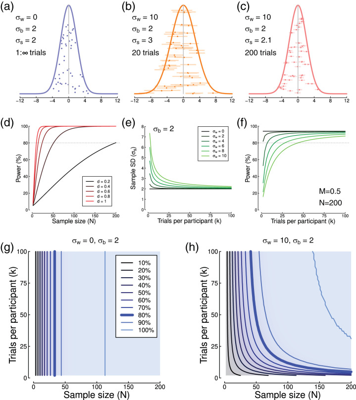
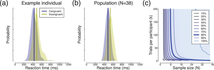
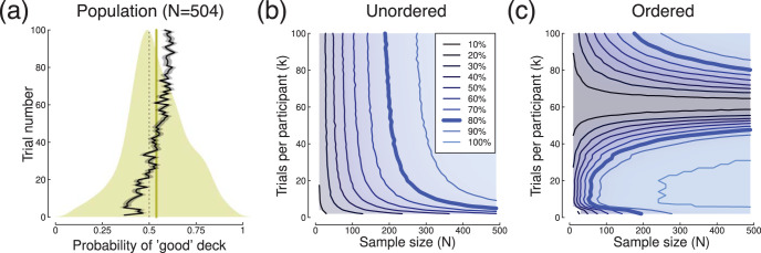
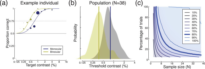
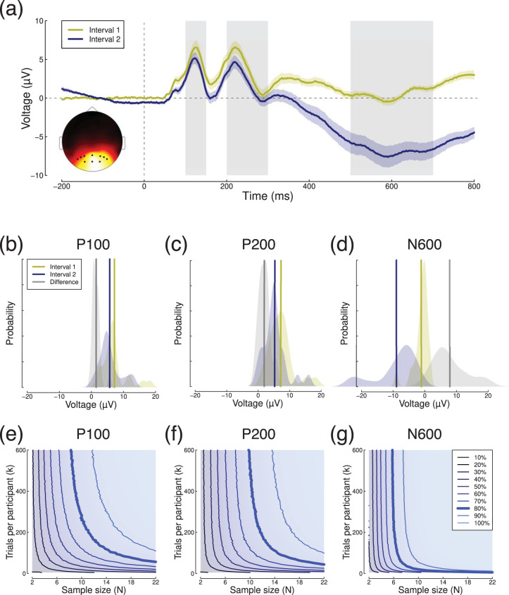
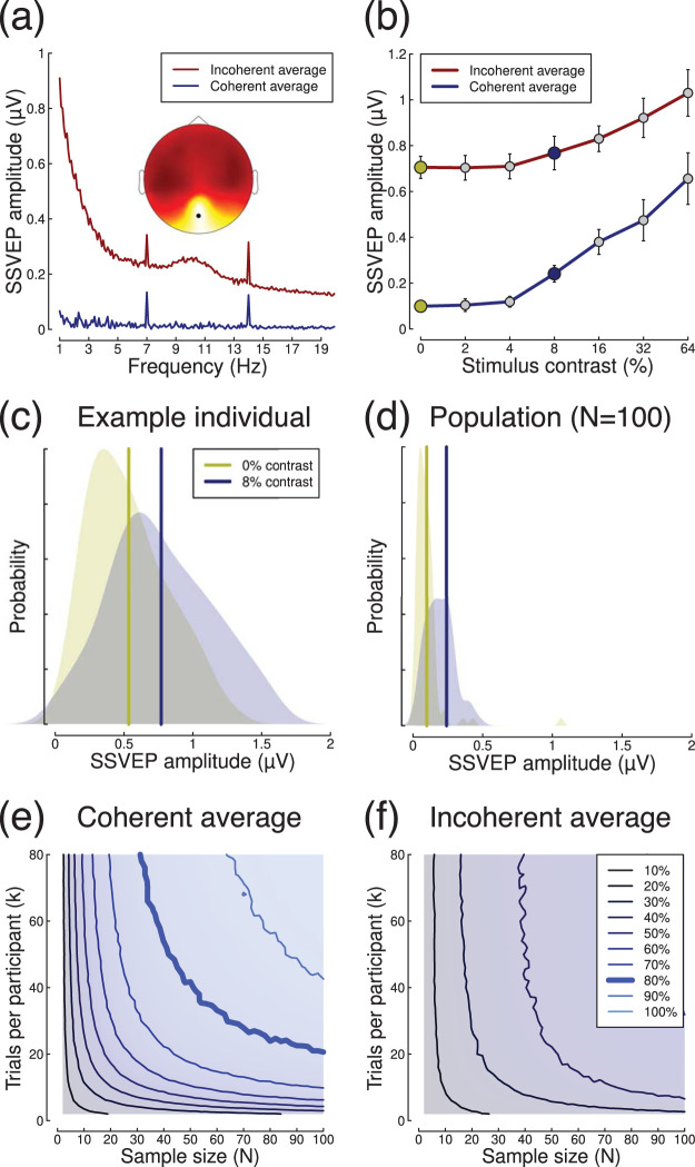
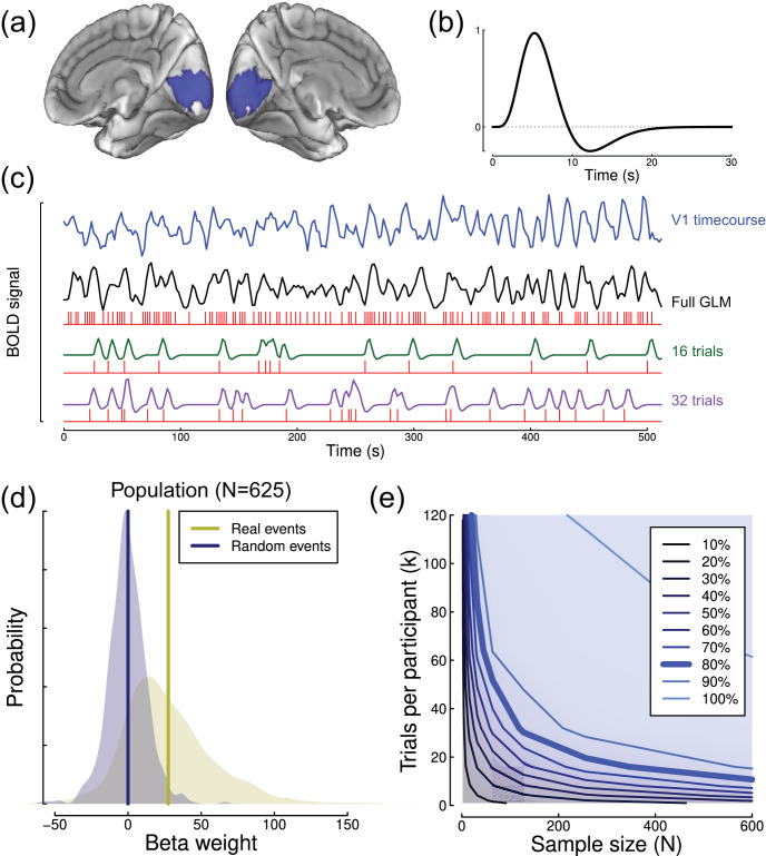
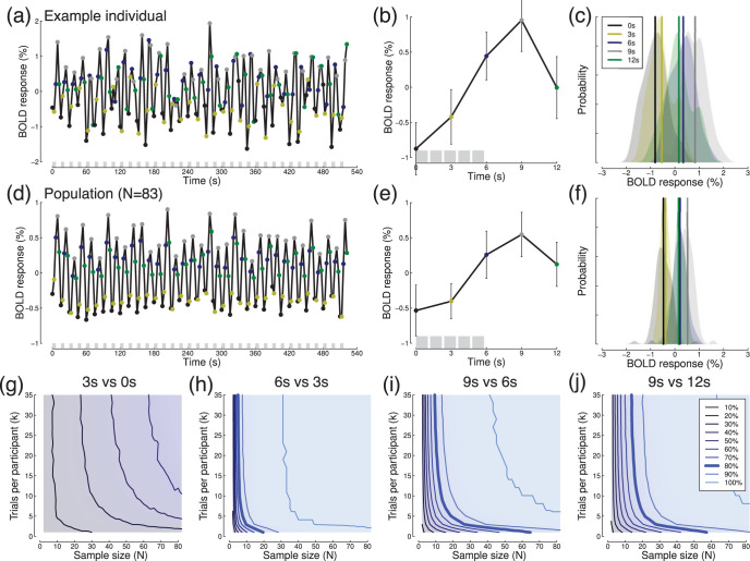
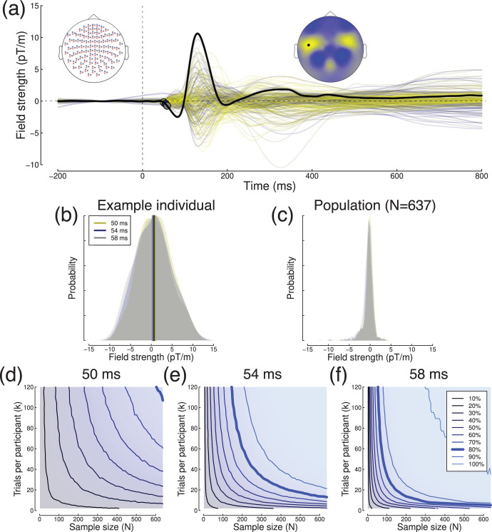
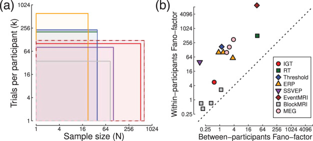
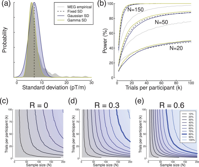
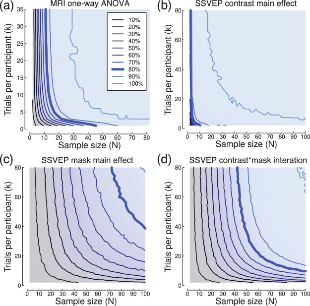
When designing experimental studies with human participants, experimenters must decide how many trials each participant will complete, as well as how many participants to test. Most discussion of statistical power (the ability of a study design to detect an effect) has focused on sample size, and assumed sufficient trials. Here we explore the influence of both factors on statistical power, represented as a 2-dimensional plot on which iso-power contours can be visualized. We demonstrate the conditions under which the number of trials is particularly important, that is, when the within-participant variance is large relative to the between-participants variance. We then derive power contour plots using existing data sets for 8 experimental paradigms and methodologies (including reaction times, sensory thresholds, fMRI, MEG, and EEG), and provide example code to calculate estimates of the within- and between-participants variance for each method. In all cases, the within-participant variance was larger than the between-participants variance, meaning that the number of trials has a meaningful influence on statistical power in commonly used paradigms. An online tool is provided (https://shiny.york.ac.uk/powercontours/) for generating power contours, from which the optimal combination of trials and participants can be calculated when designing future studies. (PsycInfo Database Record (c) 2021 APA, all rights reserved).

Figure 1

Simulations of standard deviation and statistical power. Panel (a) shows simulated data for 50 individuals, generated using a population mean of M = 0, a within-participants standard deviation of σ_w = 0, a between-participants standard deviation of σ_b = 2, and a sample standard deviation of σ_s = 2. Individual data points have a random vertical offset for display purposes. In panel (b) the within-participant standard deviation was increased to σ_w = 10, and each point is the mean of 20 trials, with horizontal error bars indicating ±1 SEM. Panel (c) shows the effect of increasing to 200 trials per participant. Panel (d) plots traditional power curves for different effect sizes (Cohen’s d) as a function of sample size (N). The dashed horizontal line indicates a power of 80%, which is generally considered acceptable. Panel (e) shows how the sample standard deviation (σ_s) depends on the number of trials per participant (k) for a range of within-participant standard deviations (see legend), and a between-participants standard deviation of σ_b = 2. Panel (f) shows the statistical power resulting from the values in panel (e), for a sample size of N = 200 and an underlying mean of M = 0.5. Panels (g, h) show power contours for different combinations of σ_w and σ_b, as described in the text, and a group mean of M = 1. Simulations used normally distributed random numbers, and statistical power was calculated for a two-sided, one-sample t test comparing to a mean of 0.

Figure 2

Summary of RT data. Panel (a) shows RT distributions for an example participant, with vertical lines giving the means. Panel (b) shows the group level data for mean RTs across the sample of 38 participants. Panel (c) shows a power contour plot, in which color represents statistical power (see legend). The thick blue line indicates combinations of sample size and trial number with a power of 80%. The y-axis represents the number of trials in the incongruent condition (the congruent condition contained three times as many trials).

Figure 3

Summary of proportion data from the Iowa Gambling task. Panel (a) shows a density plot of the mean probability of choosing a card from a “good” deck for the population of N = 504 participants, each averaged across k = 100 trials. The vertical yellow line shows the grand mean, and the dashed vertical line is the probability expected by chance. The black curve (with gray shading showing ±1 SE) shows the mean probability across all participants on each trial (1 to 100). Panel (b) shows power contours for one-sample t tests comparing the mean probability to the chance baseline (0.5). For these simulations, trials were randomly subsampled. Panel (c) shows power contours when trials were included sequentially.

Figure 4

Summary of threshold psychophysics data. Panel (a) shows psychometric functions for a single participant, with symbol size proportional to the number of trials at each target contrast level. Curves are fitted cumulative Gaussian functions, used to interpolate thresholds at 75% correct (dashed line). Data for the monocular condition (blue) were pooled across the left and right eye conditions before fitting. Panel (b) shows distributions of monocular (blue) and binocular (yellow) detection thresholds across a group of N = 38 participants with normal vision. Panel (c) shows the power contours derived by subsampling the data and refitting the psychometric functions.

Figure 5

Summary of ERP results. Panel (a) shows grand mean ERPs in response to central presentation of a 50% contrast sine wave grating in two intervals of each trial. Shaded regions surrounding each trace show ±1 SE across participants (N = 22), and the gray rectangles illustrate the time windows used to estimate peaks. The inset shows the distribution of voltages across the scalp at 226 ms after stimulus onset and black symbol mark the electrodes (Oz, O1, O2, POz, PO3–PO8) over which ERPs were averaged. Panels (b–d) show average peak voltages across a group of N = 22 participants in each time window, for both intervals and their difference. Panels (e–g) show power contours for the peak voltage within each time window.

Figure 6

Summary of SSVEP data. Panel (a) shows Fourier spectra for full 10 s long trials, using either coherent (blue) or incoherent (red) averaging, and the scalp distribution of activity at 7 Hz (inset). Panel (b) shows contrast response functions for both types of averaging. Panel (c) shows the distribution of amplitudes for an example participant, and panel (d) shows averages for the population. Panels (e) and (f) show power contours for coherent and incoherent averaging, respectively.

Figure 7

Summary of event-related fMRI analysis and results. Panel (a) shows the V1 region of interest on the medial surface of the standard (MNI152) brain, highlighted in blue. Panel (b) shows the canonical double gamma hemodynamic response function used in our general linear models. Panel (c) shows an example time-course from the V1 ROI for one participant (blue), and a general linear model constructed to predict this time-course (black) based on stimulus events (red). The green and purple traces show example GLM components with random subsets of trials. Panel (d) shows the population distributions of beta weights for the full GLM modeling all stimulus events (yellow) or randomly simulated times (blue). Panel (e) shows the power contour plot for these event-related fMRI data.

Figure 8

Summary of blocked design fMRI data. Panel (a) shows an fMRI time-course for an example individual, averaged across the V1 ROI (see Figure 7a). Shaded gray regions at the foot of the panel indicate blocks when stimuli were presented. Panel (b) shows the data from panel (a) aligned to each block onset and averaged across all k = 35 blocks (with error bars showing ±1 SD). The gray shaded regions at the foot of the panel indicate the presentations of individual stimuli within a block. Panel (c) shows distributions of BOLD activity at each time point. Panels d–f mirror panels a–c but for the sample of N = 83 participants. Panels g–j show power contours for the fMRI data, comparing activity at successive time points.

Figure 9

Summary of MEG results. Panel (a) shows a butterfly plot of evoked responses from 204 planar gradiometers, averaged across all participants (N = 637). The MEG montage is depicted in the upper left inset, where planar gradiometers of orthogonal orientations are indicated in blue and red, and magnetometer locations are shown in gray. The upper right inset shows the distribution of field strengths across a subset of 102 gradiometers with consistent orientation at 130 ms (the peak of the black curve), and the black dot indicates the location of the sensor used for the analysis. Colored points highlighted on the black curve indicate time points used for power analysis. Panel (b) shows distributions of field strengths at each of the three target time points for an individual participant. Panel (c) shows the same but for the sample population of N = 637 participants. Panels (d–f) show power contours for different time-points.

Figure 10

Summary of sample sizes, trial numbers, and Fano-factors across experimental paradigms. Each rectangle in (a) covers the range of sample sizes and trial numbers for one of the studies analyzed here, with colors defined in the legend in panel (b). Panel (b) plots Fano-factors (variance divided by the mean) derived from the within- and between-participants standard deviations given in Table 1. Note the log-scaled axes for both panels.

Figure 11

Summary of the influence on power of the distribution of within-participant standard deviations, and the correlation between repeated measures. Panel (a) illustrates possible distributions of within-participant standard deviations. The gray curve shows an empirical distribution derived from the MEG data set (N = 637 at 58 ms). The dashed line gives a fixed value, which is the mean of the empirical distribution excluding values >15 pT/m. The blue curve shows a normal distribution, with mean and SD derived from the empirical distribution (M = 6.99, SD = 2.17). The yellow curve shows the gamma distribution that best fits the empirical distribution (shape = 17.64, scale = 0.36). Panel (b) shows statistical power as a function of the number of trials for a range of sample sizes, using the four distributions shown in (a). Panels (c–e) show simulated power contours for repeated measures designs as a function of the correlation (R) between the two conditions. For these simulations we assumed a group mean difference of 0.5, between participants standard deviation of 2, and within participant standard deviation of 10. The total variance remained constant across the range of correlations.

Figure 12

Example power contours for one-way and factorial ANOVAs. Panel (a) shows a power contour plot for a one-way repeated measures ANOVA using three levels from the blocked fMRI data (summarized in Figure 8). Panels (b–d) show power contours for the main effects of contrast (b) and mask level (c), as well as their interaction (d) in a 7 × 2 repeated measures ANOVA design using the SSVEP data set (summarized in Figure 6).

References

1. Baker D. H., Lygo F. A., Meese T. S., & Georgeson M. A. (2018). Binocular summation revisited: Beyond 2. Psychological Bulletin, 144, 1186–1199. 10.1037/bul0000163 - DOI - PMC - PubMed
1. Bishop D. (2019). Rein in the four horsemen of irreproducibility. Nature, 568, 435. 10.1038/d41586-019-01307-2 - DOI - PubMed
1. Boudewyn M. A., Luck S. J., Farrens J. L., & Kappenman E. S. (2018). How many trials does it take to get a significant ERP effect? It depends. Psychophysiology, 55, e13049. 10.1111/psyp.13049 - DOI - PMC - PubMed
1. Boynton G. M., Engel S. A., Glover G. H., & Heeger D. J. (1996). Linear systems analysis of functional magnetic resonance imaging in human V1. Journal of Neuroscience, 16, 4207–4221. - PMC - PubMed
1. Brandmaier A. M., von Oertzen T., Ghisletta P., Hertzog C., & Lindenberger U. (2015). Lifespan: A tool for the computer-aided design of longitudinal studies. Frontiers in Psychology, 6, 272. 10.3389/fpsyg.2015.00272 - DOI - PMC - PubMed