A Neural Network for Wind-Guided Compass Navigation

Abstract

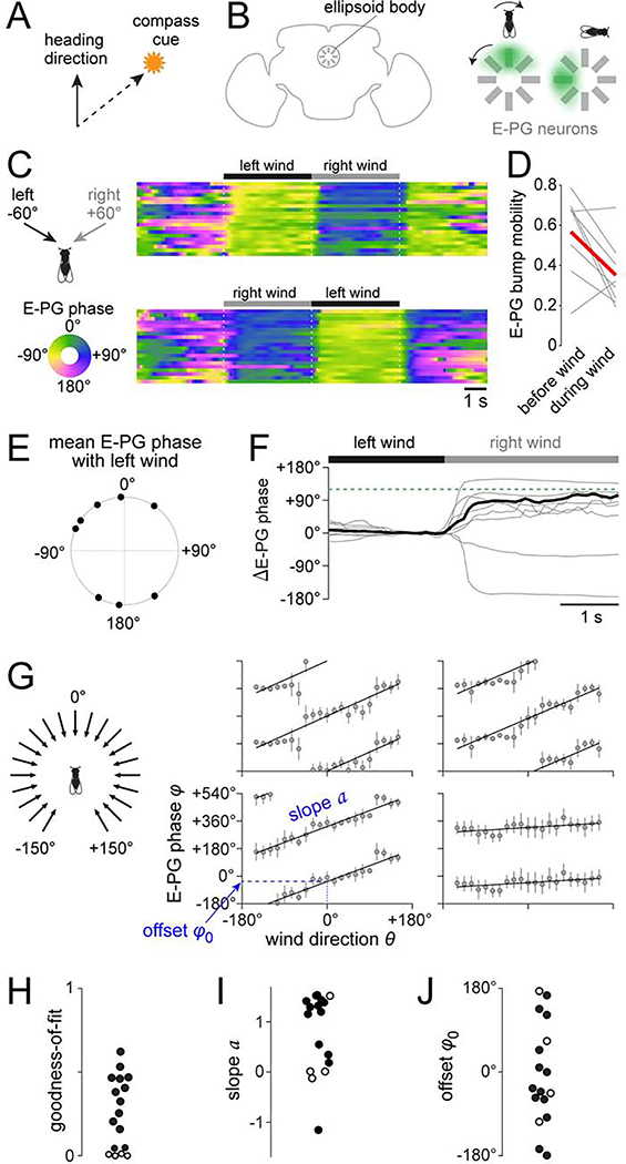
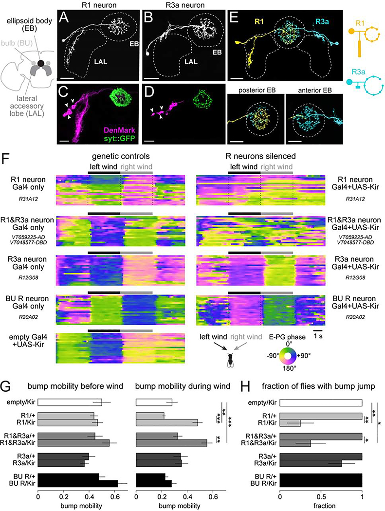
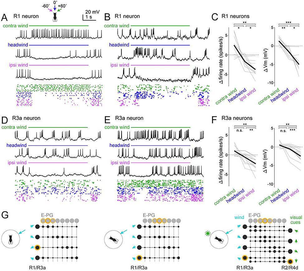
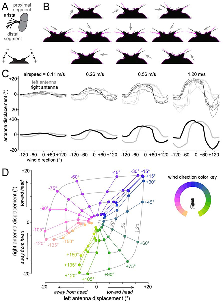
Spatial maps in the brain are most accurate when they are linked to external sensory cues. Here, we show that the compass in the Drosophila brain is linked to the direction of the wind. Shifting the wind rightward rotates the compass as if the fly were turning leftward, and vice versa. We describe the mechanisms of several computations that integrate wind information into the compass. First, an intensity-invariant representation of wind direction is computed by comparing left-right mechanosensory signals. Then, signals are reformatted to reduce the coding biases inherent in peripheral mechanics, and wind cues are brought into the same circular coordinate system that represents visual cues and self-motion signals. Because the compass incorporates both mechanosensory and visual cues, it should enable navigation under conditions where no single cue is consistently reliable. These results show how local sensory signals can be transformed into a global, multimodal, abstract representation of space.

Keywords: AMMC; Johnston’s organ; Ring neuron; central complex; ellipsoid body; lateral accessory lobe; mechanosensation; sensorimotor integration; wedge.

Figure 1.. Wind influences the brain’s heading compass.

(A) Schematic of compass behavior. Animals can maintain a straight course by keeping a fixed angle between their heading and a compass cue. (B) Schematic of E-PG neuron dendrites, which form a circular array in the ellipsoid body. A “bump” of activity (green shading) rotates as the fly turns. (C) Heat map of E-PG phase (i.e. bump position) as we delivered wind from −60° or +60°. Each row is a different trial. (D) E-PG bump mobility quantifies how much the bump moves over time. We computed mobility within each trial during the baseline period (“before wind”). We computed mobility separately for each wind direction, and then averaged these values (“during wind”). Each gray line indicates one fly and red is the mean across all the flies. Wind significantly decreased bump mobility in 6 of 8 flies; it had the opposite effect in one fly, and no significant effect in one fly; significance assessed at criterion of 0.05, Wilcoxon rank-sum tests). (E) Mean E-PG phase during wind from −60°. Each symbol is a fly (n=8). The distribution of phases was not significantly different from uniform (p = 0.61, Rayleigh test). (F) Change in E-PG phase during the wind shift from left to right, expressed as a change from baseline (0–1 s before the wind shift). Each gray line is trial-averaged data for one fly, and the black line is mean across flies (n=8). Dashed line indicates 120°, which was the separation between left and right wind. (G) Mean E-PG phase verus wind direction for four flies, with fits to φ = [a ·θ + φ₀] (mod 360°). Error bars show angular deviation. See Figure S1F for all flies. (H) Goodness-of-fit of the linear model. Each symbol is a fly. Fit was statistically significant in 13 flies (solid symbols) and not significant in 4 flies (open symbols). The same 4 flies are marked with open symbols in (I) and (J). (I) Value of the slope a. (J) Value of the offset φ₀ between the wind and the bump.

Figure 2.. The influence of wind on E-PG neurons requires R1 neurons.

(A) Single-cell labeling of an R1 neuron using MultiColor FlpOut (MCFO). (B) MCFO labeling of an R3a neuron. Both R1 and R3a have smooth neurites in the LAL and boutons in the EB. (C) In R1 neurons, DenMark localizes to the LAL, whereas synaptotagmin::GFP localizes to the EB. LAL labeling is bilaterally symmetric, but only one LAL is shown. Arrowheads indicate somata. (D) Same but for R3a neurons. (E) Simultaneous two-color labeling of an R1 and R3a neuron using MCFO. R1 innervates the posterior EB; R3a innervates the anterior EB. Schematic at right compares R1 and R3a neuron morphologies. (F) Heat map of the E-PG phase (i.e. bump location) as we delivered wind from −60° and +60°. Shown are 9 example flies, one per genotype. Within a block, each row is a trial. (G) E-PG bump mobility before wind (left) and during wind (right), for each genotype, mean ± SEM across flies (n = 8 flies per genotype). Before wind, there is no significant difference between the Gal4/+ and Gal4/Kir conditions (two-way ANOVA with Gal4 line as one factor and the presence of Kir as another factor, p=0.09). During wind, there is a significant difference between the Gal4/+ and Gal4/Kir conditions (two-way ANOVA with Gal4 line as one factor and Kir as another factor, p=9.2×10–6) and the interaction term is also significant (p=0.004). Asterisks show results from post-hoc two-sample t-tests. See Figure S2J for individual flies. (H) Fraction of flies where a wind direction switch evoked a significant E-PG phase change; mean ± SEM across flies, n = 8 flies per genotype. Fisher’s exact test. *p<0.05, **p<0.01, ***p<0.001. Scale bars in (A)-(E) are 20 μm.

Figure 3:. R1 and R3a neurons show direction-selective wind responses.

(A) R1 neuron responses to three wind directions. Raster plots show 10 randomly chosen trials. (B) Same but for another R1 neuron with different tuning. (C) Responses of all R1 neurons. Within each panel, each gray line is a neuron (1 per fly), black line is the mean across flies. Responses are averaged over the entire stimulus period and all trials and are expressed as changes from baseline. Responses depended on wind direction for both firing rate (p=2.4×10⁻⁴) and membrane potential (p=9.7×10⁻⁶); both tests one-way repeated measures ANOVA followed by paired t-tests with Bonferroni corrections; n = 9 neurons. (D-F) Same as (A-C) but for R3a. Responses depended on wind direction for both firing rate (p=1.3×10⁻⁴) and membrane potential (p=3.5×10⁻⁵); both tests one-way repeated measures ANOVA followed by paired t-tests with Bonferroni corrections; n = 12 neurons. R1 and R3a are significantly different (p=0.006, two-way repeated measures ANOVA with R1/R3a as one factor and wind direction as the within-subject factor, interaction between neuron type and wind direction). *p<0.05, **p<0.01, ***p<0.001 (G) Model of R→E-PG connectivity. Each R neuron inhibits a subset of E-PG neurons, disinhibiting other E-PG neurons. R neurons with adjacent preferred wind directions target adjacent E-PG subsets. Co-activated mechanosensory R neurons (R1/R3a neurons) and visual R neurons (R2/R4d neurons) connect to the same E-PG neurons. Active neurons are highlighted in yellow. Synaptic weights are represented as circles, with larger circles denoting larger weights (stronger inhibition).

Figure 4:. Antennal mechanics are nonlinearly sensitive to lateral wind directions.

(A) Top: schematic of the arista and antenna in frontal-medial view. Wind exerts force on the arista and rotates the distal antennal segment relative to the proximal segment. Bottom: schematic of the head in dorsal view. Wind can push the antenna toward (+) or away from the head (−). (B) Dorsal view of the antennae with resting position in black, and wind-induced positions in magenta. Arrows are wind direction (wind speed: 1.20 m/s). (C) Antennal displacements as a function of wind direction and wind speed. Top: individual flies. Bottom: mean across flies. (D) Data from one fly in (C), displayed as trajectories in 2-D displacement space. In this plot, we pooled mirror-reflected data from the left and right to generate a symmetric map. Data points are color-coded by wind direction. Displacements measured at the same wind speed are connected, with the corresponding wind speeds (m/s) in gray type.

Figure 5:. R1 and R3a neurons combine displacement signals from both antennae.

(A) Example recording of an R1 neuron in the left hemisphere. Antennal displacements were ordered pseudo-randomly, and were maintained for 1 -s periods, with ramps in between. (B) Top: responses of an R1 neuron in the left hemisphere to unilateral stimuli (i.e., stimuli where one antenna was displaced while holding the other antenna was held in its resting position). The horizontal line is this cell’s mean firing rate when both antennae are at rest (±95% confidence interval). Bottom: same for another R1 neuron in the left hemisphere. Whereas cell 1 is more sensitive to the ipsilateral antenna, cell 2 is more sensitive to the contralateral antenna. (C) Left: scatterplots show responses of the same two R1 neurons, for all tested combinations of left and right displacements. Right: continuous maps obtained by 2D-interpolation of these scatterplots. (D) Predicted bilateral responses of the same two R1 neurons, obtained by linearly combining each cell’s responses to unilateral stimuli alone, and then interpolating. See Figure S4 for other R1 neurons and R3a neurons. (E) Estimated wind direction tuning curves of the same two example R1 neurons, at three different wind speeds. The transformation from antennal coordinates to wind coordinates was calculated from the measurements in Figure 4D. (F) Estimated wind direction tuning curves for five recorded R1 neurons (wind speed 0.56 m/s). (G) Estimated wind direction tuning curves for two recorded R3a neurons.

Figure 6:. R neuron tuning reflects antennal mechanics, whereas E-PG neuron tuning does not.

(A) Schematic: we used calcium imaging to monitor R1 somata while delivering wind from 21 angles in pseudo-random order. (B) Maximum z-projection showing R1 somata in the left brain and corresponding ROIs. (C) Time course of ΔF/F responses to several wind directions for these same ROIs. (D) ΔF/F versus wind direction for R1 neurons in the left brain, and also for the right brain in the same individual. See Figure S5A for all R1 soma imaging experiments. (E) Antennal displacement versus wind direction for a typical experiment (Figure 4). The right axis is inverted; this follows the preferences of left brain R1 neurons, which are excited when the left antenna is moved toward the head or the right antenna is moved away from the head. (F) R1 tuning curves from (D), normalized so all curves have the same range. Overlaid are model fits. The only free parameters in the model were the weights of the curves in (E). (G) E-PG tuning curves from an example experiment (from Figure 1). (H) Schematics showing an individual R1 neuron forming potential synapses with every E-PG dendrite (left) and a matrix of patterned R1→E-PG connection weights (right). (I) Response probabilities of model E-PG neurons, modeled as binary units. R1→E-PG weights are adjusted to maximize the probability that each E-PG neuron responds to its target heading while minimizing its responses to other headings.

Figure 7:. R1 neurons receive direct GABAergic inhibition from WL-L neurons.

(A) MCFO labeling of an WL-L neuron, showing smooth neurites in the ipsilateral WED and ipsilateral LAL, and boutons in the contralateral LAL. Scale bars in (A-C) are 50 μm. (B) Two-color MCFO labeling of two WL-L neurons in the same brain. Note that each cell’s bouton-rich arbor is just medial to the smooth arbor of the contralateral cell. (C) Polarity markers expressed in WL-L neurons. The dendritic marker DenMark localizes to smooth arbors, whereas synaptotagmin::GFP localizes to bouton-rich arbors. Dashed lines indicate synaptotagmin::GFP in another cell type in the same Gal4 line (not WL-L). (D) Recording from a CsChrimson+ WL-L neuron. Left: light-evoked response in an example trial (enlarged in inset). Right: firing rates in 3 neurons (in 3 flies). Green bars indicate 10-ms light pulses. (E) Recording from R1 neurons while activating WL-L neurons. Responses were recorded first without antagonists, then in 1 μM TTX, and then after adding 5 μM picrotoxin (retaining TTX). Stimulus intensity was increased after adding TTX, to compensate for decreased excitability of presynaptic terminals. Left: single-trial responses from one neuron. Middle: trial-averaged responses for the same neuron. Right: trial-averaged responses for all neurons (n=11, 7, 4 neurons for the top, middle, and bottom rows).

Figure 8:. WL-L neurons encode unilateral antennal displacement and contribute to R1 wind responses.

(A) An example whole-cell recording from an WL-L neuron in response to wind from −60°, 0°, and +60°. (B) Same as (A) but with only the contralateral antenna intact. (C) Same as (A) but with only the ipsilateral antenna intact. Here, excitation in response to contralateral wind is abolished. Inhibition in response to ipsilateral wind has also been abolished and is replaced by weak excitation. (D) WL-L summary data. Responses are averaged over the stimulus period and expressed as changes from baseline. Within each condition, a gray line is a fly. The interaction between the stimulus (−60°, 0°, +60°) and the antennal condition (both, contra, ipsi) was not significant comparing “both-antennae-intact” with “contra-antenna-intact” (p=0.87), but it was significant comparing “both-antenna-intact” with “ipsi-antenna-intact” (p = 0.0006; two-way repeated measures ANOVA). (E) Recording from a GtACR1+ WL-L neuron. Light (620 nm, 4.5 s) hyperpolarizes the neuron and suppresses spiking. (F) R1 recording to test the effect of silencing WL-L neurons using GtACR1. We measured responses to wind from +60°, 0°, and 60°, with and without light. (G) Mean membrane potential of the same R1 neuron (mean ± SEM; 8 trials per condition). (H) Summary of wind responses in R1 neurons with and without WL-L silencing. Responses are averaged over the stimulus period and expressed as changes from baseline. Each line is a different neuron (n = 5). The effect of light is significant for ipsilateral wind (p=0.003; paired t-test). Also plotted is the mean response to light alone (no wind); note that light alone is depolarizing, implying that WL-L neurons are tonically inhibiting R1 neurons. Figure S7G-I shows data for genetic controls (lacking GtACR expression). (I) Schematic showing the cell types involved in the transformation from wind-induced antennal displacements to compass signals. Filled circle, bar, and resistor symbols indicate excitatory connections, inhibitory connections, and gap junctions, respectively.

References

1. Alvarez-Salvado E, Licata AM, Connor EG, McHugh MK, King BM, Stavropoulos N, Victor JD, Crimaldi JP, and Nagel KI (2018). Elementary sensory-motor transformations underlying olfactory navigation in walking fruit-flies. eLife 7. - PMC - PubMed
1. Amit DJ, Wong KYM, and Campbell C (1989). Perceptron learning with sign-constrained weights. J Phys A-Math Gen 22, 2039–2045.
1. Awasaki T, Lai SL, Ito K, and Lee T (2008). Organization and postembryonic development of glial cells in the adult central brain of Drosophila. J Neurosci 28, 13742–13753. - PMC - PubMed
1. Baker DA, Beckingham KM, and Armstrong JD (2007). Functional dissection of the neural substrates for gravitaxic maze behavior in Drosophila melanogaster. J Comp Neurol 501, 756–764. - PubMed
1. Bates AS, Franconville R, and Jefferis GSXE (2019a). neuprintr: R client utilities for interacting with the neuPrint connectome analysis service. R package version 0.4.0.
Publication types
LinkOut - more resources