. 2021 Jan;39(1):105-114.
doi: 10.1038/s41587-020-0603-3. Epub 2020 Jul 20.

A unified catalog of 204,938 reference genomes from the human gut microbiome

Affiliations

A unified catalog of 204,938 reference genomes from the human gut microbiome

Alexandre Almeida et al. Nat Biotechnol. 2021 Jan.

Abstract

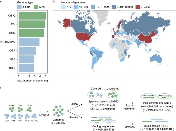
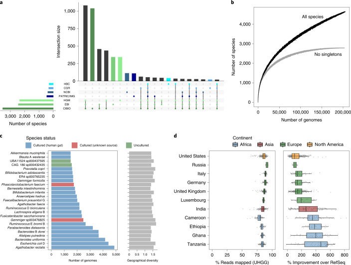
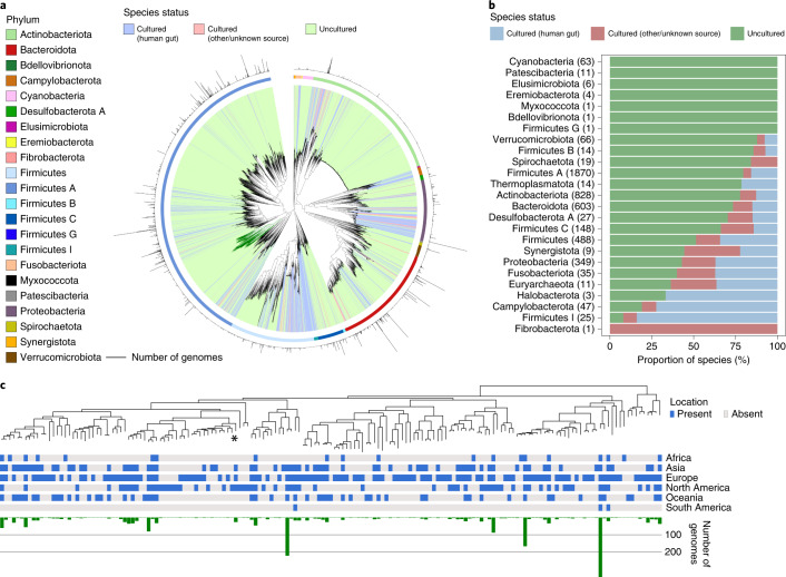
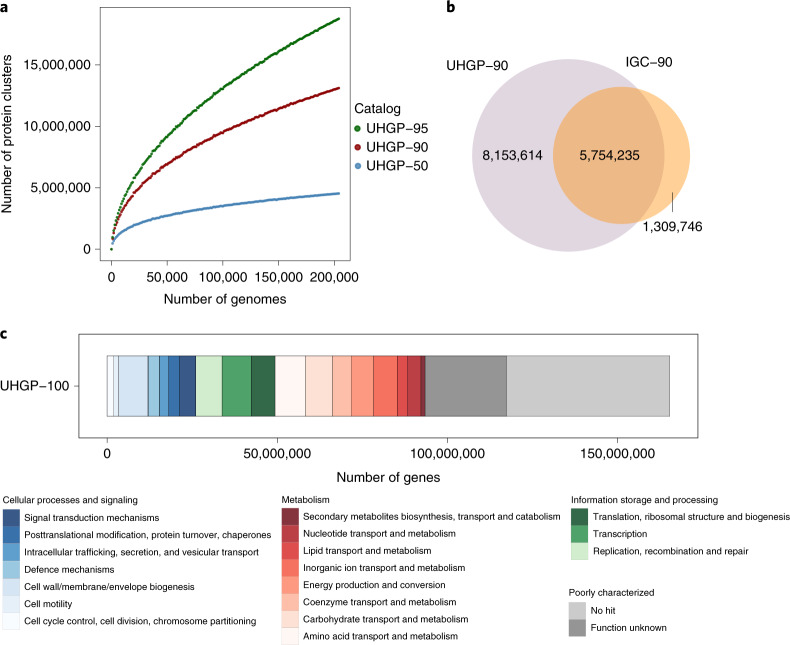
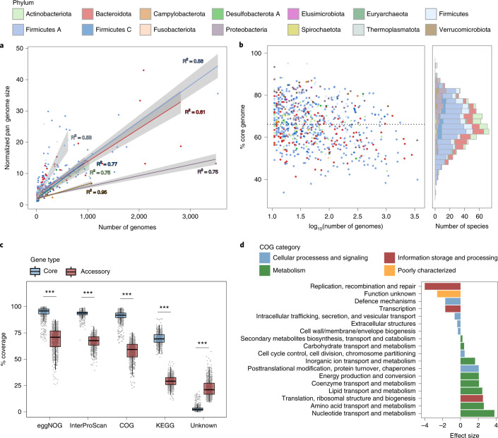
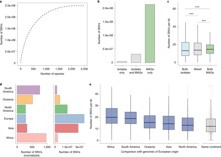
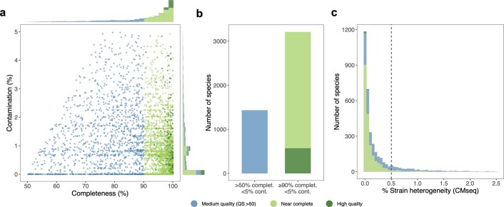
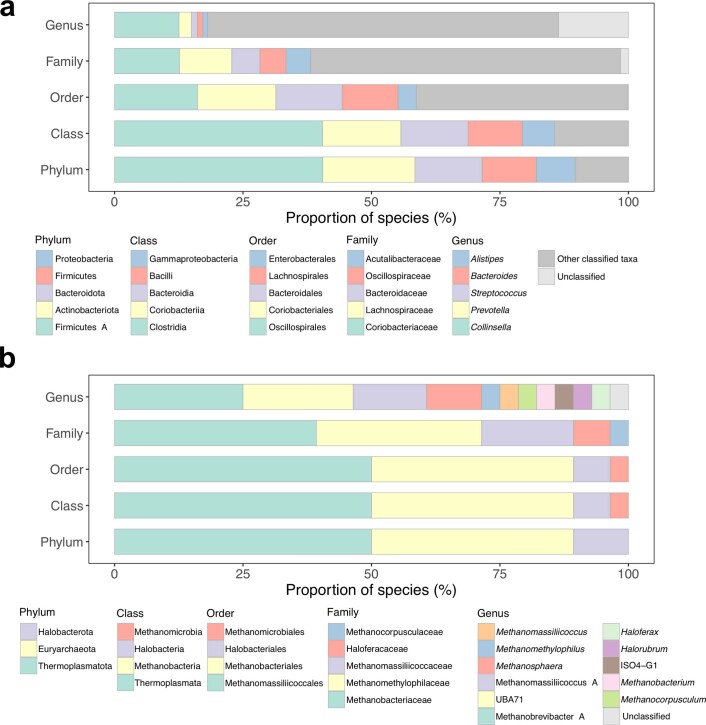
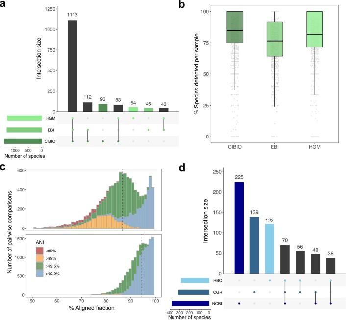
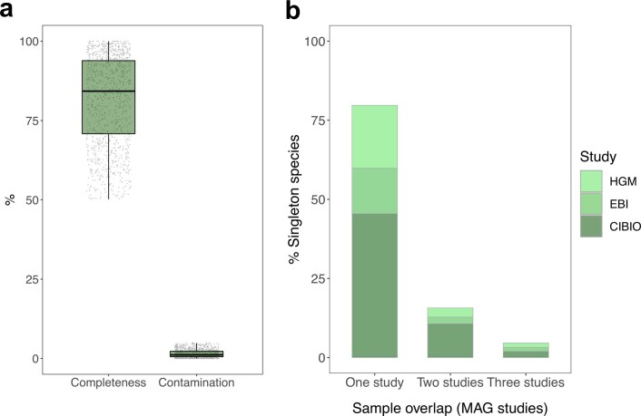
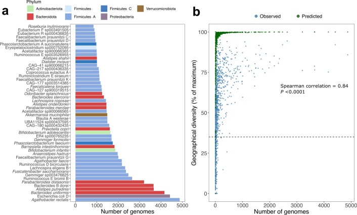
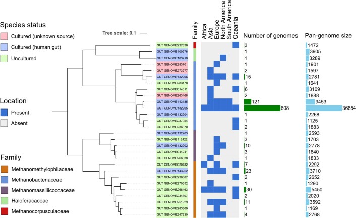
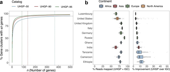
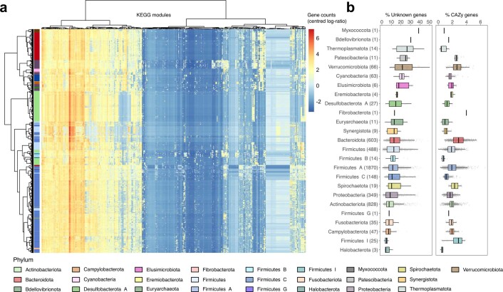
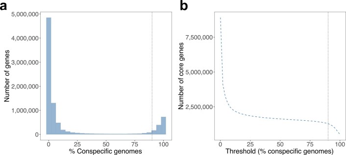
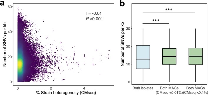
Comprehensive, high-quality reference genomes are required for functional characterization and taxonomic assignment of the human gut microbiota. We present the Unified Human Gastrointestinal Genome (UHGG) collection, comprising 204,938 nonredundant genomes from 4,644 gut prokaryotes. These genomes encode >170 million protein sequences, which we collated in the Unified Human Gastrointestinal Protein (UHGP) catalog. The UHGP more than doubles the number of gut proteins in comparison to those present in the Integrated Gene Catalog. More than 70% of the UHGG species lack cultured representatives, and 40% of the UHGP lack functional annotations. Intraspecies genomic variation analyses revealed a large reservoir of accessory genes and single-nucleotide variants, many of which are specific to individual human populations. The UHGG and UHGP collections will enable studies linking genotypes to phenotypes in the human gut microbiome.


Conflict of interest statement

F.S. is an employee of Enterome. P.H. is a cofounder and is director of Microba Life Sciences Ltd. D.H.P. is a consultant to Microba Life Sciences Ltd. R.D.F. is a consultant to Microbiotica Pty Ltd.

Figures

Fig. 1
Fig. 1. The unified sequence catalog of the human gut microbiome.
a, Number of gut genomes for each study set used to generate the sequence catalogs, colored according to whether they represent isolate genomes or MAGs. b, Geographic distribution of the number of genomes retrieved per country. c, Overview of the methods used to generate the genome (UHGG) and protein sequence (UHGP) catalogs. Genomes retrieved from public datasets first underwent quality control by CheckM. Filtered genomes were clustered at an estimated species level (95% ANI), and their intraspecies diversity was assessed (genes from conspecific genomes were clustered at 90% protein identity). In parallel, a nonredundant protein catalog was generated from all coding sequences of the 286,997 genomes at 100% (UHGP-100, n = 170,602,708), 95% (UHGP-95, n = 20,239,340), 90% (UHGP-90, n = 13,907,849) and 50% (UHGP-50, n = 4,735,546) protein identity.
Fig. 2
Fig. 2. Intersection and frequency of species across studies.
a, Number of species found across genome study sets, ordered by their level of overlap. Vertical bars represent the number of species shared between the specific study sets highlighted with colored dots in the lower panel. Horizontal bars in the lower panel indicate the total number of species contained in each study set. Different shades of green denote the study sets represented exclusively by MAGs, whereas those in blue represent studies only containing isolate genomes. b, Rarefaction curves of the number of species detected as a function of the number of nonredundant genomes analyzed. Curves are depicted both for all the UHGG species and after excluding singleton species (represented by only one genome). c, Number of nonredundant genomes detected per species (left) alongside the degree of geographic diversity (calculated with the Shannon diversity index; right). Only the 25 most represented species clusters are depicted. d, Left, proportion of metagenomic reads from 1,005 independent datasets classified with Kraken 2 against the UHGG species representatives. Right, the degree of classification improvement provided over the standard Kraken 2 RefSeq database. The following correspond to the number of datasets analyzed per country: Cameroon, n = 54; Ethiopia, n = 25; Germany, n = 56; Ghana, n = 40; India, n = 105; Italy, n = 50; Luxembourg, n = 26; Russia, n = 4; Tanzania, n = 61; United Kingdom, n = 210; United States, n = 374. Box lengths represent the IQR of the data, and whiskers extend to the lowest and highest values within 1.5 times the IQR from the first and third quartiles, respectively.
Fig. 3
Fig. 3. Uncultured species are predominant among human gut phyla.
a, Maximum-likelihood phylogenetic tree of the 4,616 bacterial species detected in the human gut. Clades are colored by the cultured status of species, with outer circles depicting the GTDB phylum annotation. Bar graphs in the outermost layer indicate the number of genomes from each species. The order Comantemales ord. nov. is highlighted with dark green branches. b, Proportion of species within the 25 prokaryotic phyla detected according to cultured status. Numbers in parentheses represent the total number of species in the corresponding phylum. c, Phylogenetic tree of species belonging to the order Comantemales ord. nov. (phylum Firmicutes A), the largest phylogenetic group exclusively represented by uncultured species. The geographic distribution of each species and the number of genomes recovered are represented below the tree. The species previously classified as CandidatusBorkfalki ceftriaxensis’ is indicated with an asterisk.
Fig. 4
Fig. 4. The UHGP improves coverage of the human gut protein landscape.
a, Rarefaction curves of the number of protein clusters obtained as a function of the number of nonredundant genomes analyzed. Separate colored curves are depicted for the UHGP-95, UHGP-90 and UHGP-50. b, Overlap between the UHGP (purple) and IGC (orange), both clustered at 90% amino acid identity. c, COG functional annotation results of the unified gastrointestinal protein catalog clustered at 100% amino acid identity (UHGP-100).
Fig. 5
Fig. 5. Pan-genome diversity patterns within the gut microbiome.
a, Normalized pan-genome size as a function of the number of conspecific genomes. Regression curves were generated for each phylum, with the corresponding coefficients of determination indicated next to each curve and the shaded regions representing the 95% confidence level intervals. The following correspond to the number of species considered for each phylum: Actinobacteriota, n = 66; Bacteroidota, n = 122; Firmicutes, n = 90; Firmicutes A, n = 325; Firmicutes C, n = 44; Proteobacteria, n = 65; Verrucomicrobiota, n = 13. b, Fraction of the core genome for each species according to the number of conspecific genomes (left) and as a histogram (right), colored by phylum. The horizontal dashed line represents the median value across all species. c, Proportion of core and accessory genes (n = 781 species) classified with various annotation schemes, alongside the percentage of genes lacking any functional annotation. Box lengths represent the IQR of the data, and whiskers extend to the lowest and highest values within 1.5 times the IQR from the first and third quartiles, respectively. A two-tailed Wilcoxon rank-sum test was performed to compare the classification between the core and accessory genes (***P < 0.001). d, Comparison of the functional categories assigned to the core (n = 1,236,880) and accessory (n = 4,785,975) genes. Only statistically significant (adjusted P < 0.05) differences are shown. Significance was calculated with a two-tailed Wilcoxon rank-sum test and further adjusted for multiple comparisons using the Benjamini–Hochberg correction. A positive effect size (Cohen’s d) indicates over-representation in the core genes.
Fig. 6
Fig. 6. Analysis of intraspecies single-nucleotide variation.
a, Total number of SNVs detected as a function of the number of species. The cumulative distribution was calculated after ordering the species by decreasing number of SNVs. b, Number of SNVs detected only in isolate genomes or MAGs, or in both. c, Pairwise SNV density analysis of genomes of the same or different type (isolates, n = 808,331 comparisons; mixed, n = 1,575,895 comparisons; MAGs, n = 26,899,457 comparisons). A two-tailed Wilcoxon rank-sum test was performed to assess statistical significance and further adjusted for multiple comparisons using the Benjamini–Hochberg correction (***P < 0.001). d, Left, the number of exclusive SNVs normalized by the number of genomes per continent. Right, the number of SNVs exclusively detected in genomes from each continent. e, Pairwise SNV density analysis between genomes from Europe, the largest genome subset, and other continents. The median SNV density was calculated per species, and the distribution is shown for all species (Africa, n = 188; Asia, n = 746; North America, n = 688; Oceania, n = 35; South America, n = 151). Comparison of genomes recovered from the same continent (n = 908 species) was used as a reference. The SNV density between genomes from the same continent is significantly lower (adjusted P < 0.05) than that calculated for genomes from different continents. In c and e, box lengths represent the IQR of the data, with whiskers depicting the lowest and highest values within 1.5 times the IQR of the first and third quartiles, respectively.
Extended Data Fig. 1
Extended Data Fig. 1. Genome quality of species representatives.
a, Completeness and contamination scores for each of the 4,644 species representatives, colored by their quality classification category. Medium quality: >50% completeness; near complete: ≥90% completeness; high-quality: >90% completeness, presence of 5S, 16S and 23S rRNA genes, as well as at least 18 tRNAs. All genomes have a quality score (QS = completeness – 5 × contamination) above 50. b, Number of species according to different completeness and contamination criteria. c, Distribution of the level of strain heterogeneity (proportion of non-synonymous substitutions) estimated for the species-level MAGs using CMseq. Dashed vertical line corresponds to the threshold defined in Pasolli, et al. to distinguish medium- from high-quality MAGs.
Extended Data Fig. 2
Extended Data Fig. 2. Taxonomy composition of the bacterial and archaeal species.
a, Taxonomic affiliation of the 4,616 bacterial species detected. Data is partitioned by taxonomic rank, with only the five most highly represented taxa per rank depicted in the legend. b, Taxonomic affiliation of the 28 archaeal species detected, partitioned by taxonomic rank.
Extended Data Fig. 3
Extended Data Fig. 3. Species overlap across study sets.
a, Number of species found across the three metagenome-assembled genome sets, ordered by their level of overlap. Only those genomes recovered from the 1,554 metagenomic samples used by all three studies were considered in this analysis. b, Distribution of the proportion of species recovered per sample (n = 1,554) in each study set out of all species recovered across all three studies in the same samples. Box lengths represent the IQR of the data, and the whiskers the lowest and highest values within 1.5 times the IQR from the first and third quartiles, respectively. c, Estimated aligned fractions and average nucleotide identities (ANI) between conspecific genomes obtained in the same sample but in different MAG studies. Results for medium-quality genomes are illustrated in the top panel, whereas those for near complete (≥90% completeness) genomes are represented in the lower panel. Vertical dashed lines denote the median values. d, Number of species identified in three culture-based studies and their degree of overlap. The NCBI study set consists mainly of genomes from the Human Microbiome Project (HMP).
Extended Data Fig. 4
Extended Data Fig. 4. Quality and sample origin of uncultured singleton species.
a, Genome completeness and contamination estimates of the 1,212 uncultured species represented by a single genome. Box lengths represent the IQR of the data, and the whiskers the lowest and highest values within 1.5 times the IQR from the first and third quartiles, respectively. b, Proportion of the 1,212 singleton species, by study set, that originated from samples analysed in one, two or three of the MAG studies (CIBIO, EBI and HGM).
Extended Data Fig. 5
Extended Data Fig. 5. Species frequency and geographical diversity.
a, Number of nonredundant genomes retrieved from the 50 most highly represented species in the UHGG catalog. Each species is colored by its assigned phylum according to the figure legend. b, Geographical diversity estimated using the Shannon index in relation to the number of nonredundant genomes from each species containing more than one genome (n = 2,786). Percentage values represent the estimated diversity normalized by the maximum theoretical value (considering an equal distribution of samples across the six major continents — Africa, Asia, Europe, North America, South America and Oceania). The Spearman’s rank correlation coefficient and P value (calculated with the Spearman’s test) are depicted in the graph. Predicted values represent the random geographical distribution of equivalent numbers of genomes observed for each species. Dashed horizontal line indicates the median observed value for species with more than one genome.
Extended Data Fig. 6
Extended Data Fig. 6. Diversity of the gut archaeal species detected.
Phylogenetic tree of the 28 archaeal species detected in the human gut. Tips are labelled with the corresponding species representative code and colored according to its cultured status. The taxonomic affiliation (family), geographical distribution, number of nonredundant genomes and total pan-genome size are represented next to the tree.
Extended Data Fig. 7
Extended Data Fig. 7. UHGP cluster size and mapping rate.
a, Cumulative distribution curve of the number and size of the gene clusters of the UHGP-95 (n = 20,239,340), UHGP-90 (n = 13,907,849) and UHGP-50 (n = 4,735,546). Dashed vertical lines indicate the cluster size below which 90% of the gene clusters can be found. b, Proportion of metagenomic reads from 1,005 independent datasets aligned with DIAMOND against the combined clusters of UHGP-90 and IGC-90 (left). The degree of classification improvement provided over the IGC-90 alone is represented in the right panel. The following represents the number of datasets analysed per country: Cameroon, n = 54; Ethiopia, n = 25; Germany, n = 56; Ghana, n = 40; India, n = 105; Italy, n = 50; Luxembourg, n = 26; Russia, n = 4; Tanzania, n = 61; United Kingdom, n = 210; United States, n = 374. Box lengths represent the interquartile range (IQR) of the data, and the whiskers the lowest and highest values within 1.5 times the IQR from the first and third quartiles, respectively.
Extended Data Fig. 8
Extended Data Fig. 8. Functional annotation of gut microbiome species.
a, Functional profiles of the UHGG species pan-genomes (rows) according to 363 KEGG modules (columns). Numbers of genes matching each module were normalized to centered log ratios after imputing values with zero counts. Species are colored according to phylum. KEGG modules and species were hierarchically clustered using the Ward’s criterion method. b, Proportion of each species pan-genome, partitioned by phylum, without any assignment to the eggNOG, InterPro, COG or KEGG databases (left). Proportion of the pan-genome with a match to the carbohydrate-active enzymes (CAZy) database (right). Sample size (number of species) of each phylum is indicated in parentheses (n = 4,644 total species). Box lengths represent the IQR of the data, and the whiskers the lowest and highest values within 1.5 times the IQR from the first and third quartiles, respectively.
Extended Data Fig. 9
Extended Data Fig. 9. Gene frequency distribution within the species-level clusters.
a, Distribution of the number of genes found per fraction of conspecific genomes. Only near-complete genomes (≥90% completeness) were considered in the analysis. b, Number of core genes detected based on the threshold of genomes per species used to classify as core. Vertical dashed line represents the 90% threshold used in this study.
Extended Data Fig. 10
Extended Data Fig. 10. SNV density and MAG strain heterogeneity.
a, Correlation between the SNV density calculated among MAGs and their level of strain heterogeneity estimated with CMseq (n = 268,994 comparisons). A Pearson correlation test was performed to determine the correlation coefficient and P value. Colors denote density of data points (increasing from dark purple to yellow). b, Comparison of pairwise SNV density between isolates (n = 808,331 comparisons) and between MAGs with <0.01% (n = 2,923,610 comparisons) and <0.1% strain heterogeneity (n = 13,634,222 comparisons). A two-tailed Wilcoxon rank-sum test was performed to assess statistical significance and further adjusted for multiple comparisons using the Benjamini-Hochberg correction (***P <0.001). Box lengths represent the IQR of the data, and the whiskers the lowest and highest values within 1.5 times the IQR from the first and third quartiles, respectively.

References

    1. Qin J, et al. A metagenome-wide association study of gut microbiota in type 2 diabetes. Nature. 2012;490:55–60. - PubMed
    1. Feng Q, et al. Gut microbiome development along the colorectal adenoma–carcinoma sequence. Nat. Commun. 2015;6:6528. - PubMed
    1. Thomas AM, Segata N. Multiple levels of the unknown in microbiome research. BMC Biol. 2019;17:48. - PMC - PubMed
    1. Human Microbiome Project Consortium. Structure, function and diversity of the healthy human microbiome. Nature. 2012;486:207–214. - PMC - PubMed
    1. Li J, et al. An integrated catalog of reference genes in the human gut microbiome. Nat. Biotechnol. 2014;32:834–841. - PubMed

Publication types