. 2020 Aug 20;182(4):812-827.e19.
doi: 10.1016/j.cell.2020.06.043. Epub 2020 Jul 3.

Tracking Changes in SARS-CoV-2 Spike: Evidence that D614G Increases Infectivity of the COVID-19 Virus

Collaborators, Affiliations

Tracking Changes in SARS-CoV-2 Spike: Evidence that D614G Increases Infectivity of the COVID-19 Virus

Bette Korber et al. Cell. .

Abstract

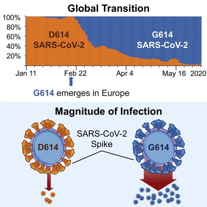
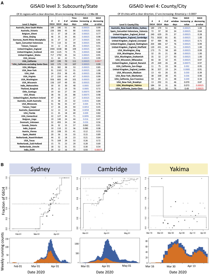
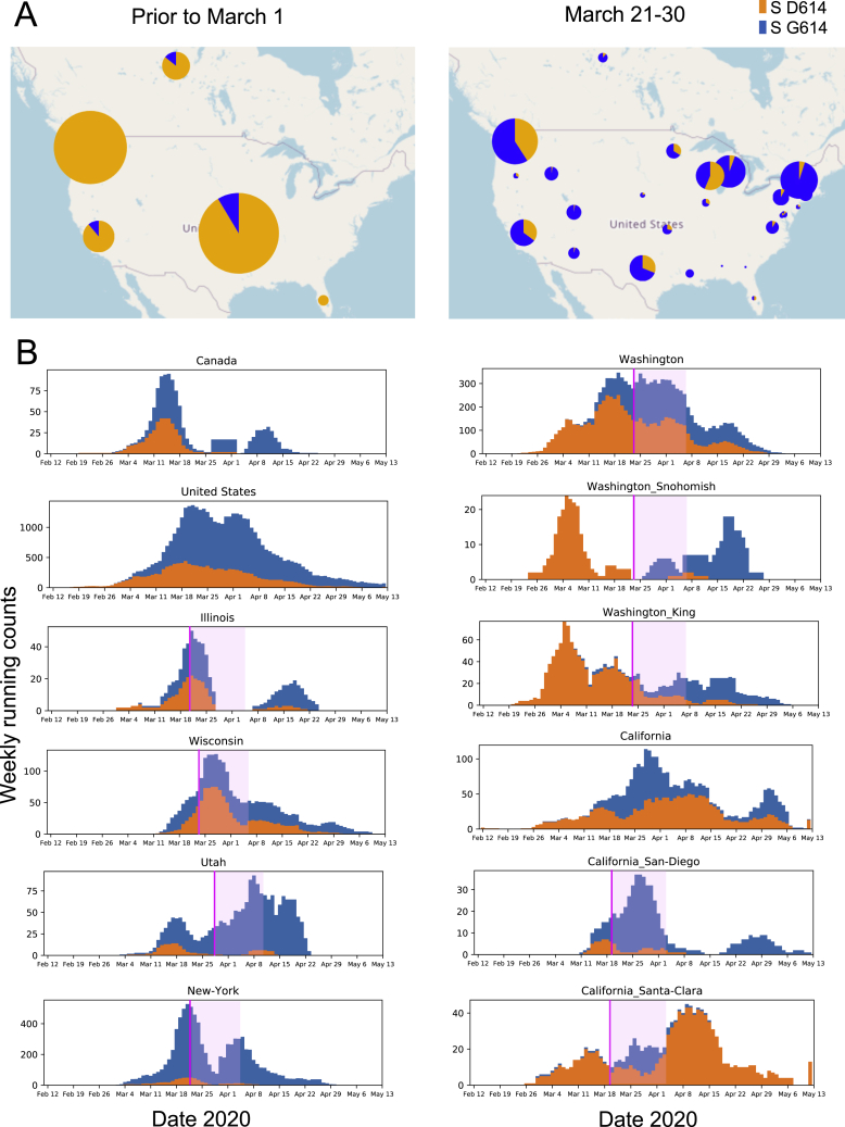
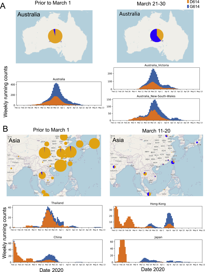
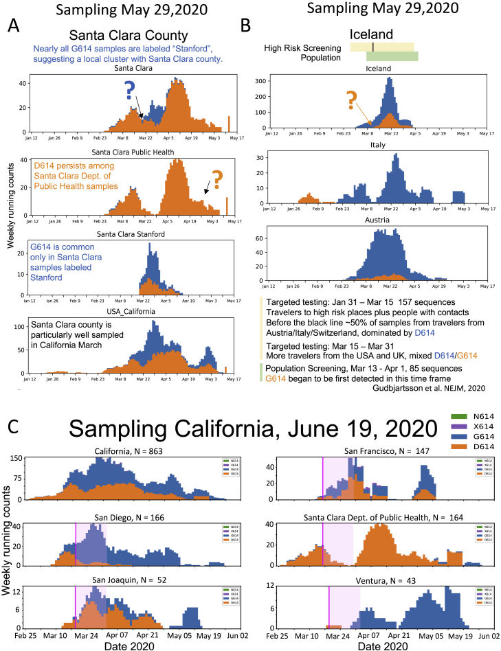
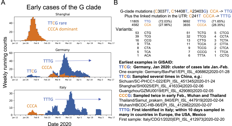
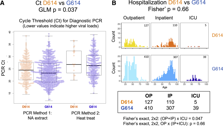
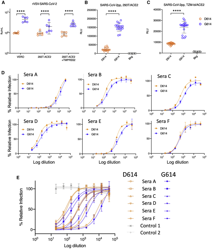
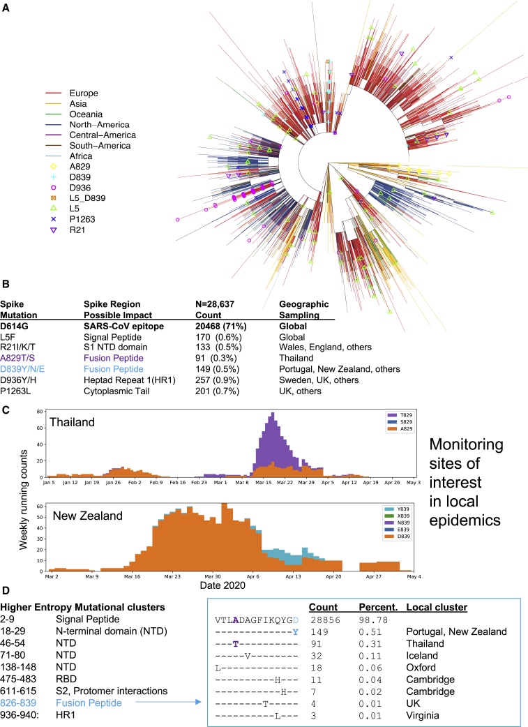
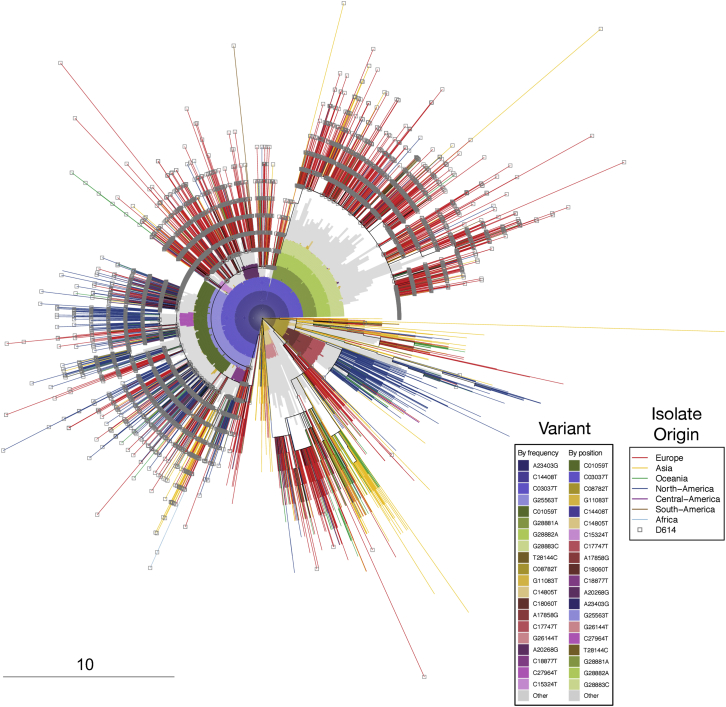
A SARS-CoV-2 variant carrying the Spike protein amino acid change D614G has become the most prevalent form in the global pandemic. Dynamic tracking of variant frequencies revealed a recurrent pattern of G614 increase at multiple geographic levels: national, regional, and municipal. The shift occurred even in local epidemics where the original D614 form was well established prior to introduction of the G614 variant. The consistency of this pattern was highly statistically significant, suggesting that the G614 variant may have a fitness advantage. We found that the G614 variant grows to a higher titer as pseudotyped virions. In infected individuals, G614 is associated with lower RT-PCR cycle thresholds, suggestive of higher upper respiratory tract viral loads, but not with increased disease severity. These findings illuminate changes important for a mechanistic understanding of the virus and support continuing surveillance of Spike mutations to aid with development of immunological interventions.

Keywords: COVID-19; PCR cycle threshold; SARS-CoV-2; Spike; antibody; diversity; evolution; infectivity; neutralization; pseudovirus.


Conflict of interest statement

Declaration of Interests The authors declare no competing interests.

Figures

None
Graphical abstract
Figure S1
Figure S1
Schematic of the SARS-CoV-2 Outbreak Sequence Processing Pipeline, Related to Figure 1 The intent of these procedures is to generate, for each of several regions, a set of contiguous codon-aligned sequences, complete in that region, without extensive uncalled bases, large gaps, or regions that are unalignable or highly divergent, in reasonable running time for n > 30,000 ∼30kb viral genomes. This allows daily processing of GISAID data to enable us to track mutations. This process provides the foundational data to enable the generation of Figures 1, 2, 3, and 7. A. Processing procedures: 1. Download all SARS-CoV-2 sequences from GISAID.org (34,607 as of 2020-05-29). The downloaded sequences are stored in compressed form (via bzip2: https://sourceware.org/git/bzip2.git). 2. Align sequences to the SARS-CoV-2 reference sequence (NC_045512), trim to desired endpoints, and filter for coverage and quality. These steps are incorporated in a single Perl script, ‘align_to_ref.pl’, briefly summarized here: sequences are compressed for identity, then mapped against the given reference sequence using ‘nucmer’ from the ‘MUMmer’ package (Kurtz et al., 2004). The nucmer ‘delta’ file contains locations of matching regions and is parsed and used to, first, partition the sequences into “good” and “bad” subsets, and then to generate alignments from the “good” sequences. B. Categories of sequences included and excluded from our automated alignments. A series of criteria is used successively to exclude sequences with large internal gaps, excessive five- and three-prime gaps, large numbers of mismatches or ambiguities (> 30) overall, or regions with a high concentration of mismatches or ambiguities (> 10 in any 100 nt subsequence): the counts of these categories of “bad” sequence are shown, for different regional genome alignments. We then create the following different regional subalignments: CODING-REGIONS2 (“FULL,” from the 5′-most start-codon (orf1ab) to the 3′-most stop-codon (ORF10), NC_045512 bases 266-29,674; SPIKE, the complete surface glycoprotein coding region, bases 21,563-25,384; NEAR-COMPLETE (“NEARCOMP,” the most-commonly-sequenced region of the genome, bases 55-29,836; COMPLETE, matching the NC_045512 sequence from start up to the poly-A tail, bases 1-29,870; 5′ UTR, the five-prime untranslated region, bases 1-265 only. Generally speaking, the smaller the region, the more sequences are included. Sequences are trimmed to the extent of the reference (with minimum allowed gaps at 5′ and 3′ ends), following which the pairwise alignments are generated from the matching regions, and a multiple sequence alignment is constructed from the pairwise alignments. 3. De-duplicate1. To reduce computational demands, sequences are compressed by identity following trimming to the desired region, by computing a hash value for each sequence (currently the SHA-1 message digest, 160 bits encoded as a 40-character hex string). To prevent the loss of parsimony-informative characters when they occur in identical strings, however, multiple sequences are reduced to a minimum of two occurrences. 4. Codon-align. Gaps are introduced into the entire compressed alignment so that the alignment column containing the last base of each codon has a number divisible by three; this simplifies processing of translations. Code for this procedure is derived from the GeneCutter tool from the LANL HIV database (https://www.hiv.lanl.gov/content/sequence/GENE_CUTTER/cutter.html). 5. Partition (full/spike-only). For subalignments that encompass the spike protein and substantial additional sequence, the spike region is extracted separately, to allow matched comparisons. 6. Build parsimony trees. A brief parsimony search (parsimony ratchet, with 5 replicates) is performed with ‘oblong’ (Goloboff, 2014) This is intended as an efficient clustering procedure rather than an explicit attempt to achieve an accurate phylogenetic reconstruction, but it appears to yield reasonable results in this situation of a very large number of sequences with a very small number of changes, where more complex models may be subject to overfitting. When multiple most-parsimonious trees are found, only the shortest of these (under a p-distance criterion) is retained. Distance scoring is performed with PAUP (Swofford, 2003). 7. Re-duplicate (expand, i.e., uncompress). The original sequence names and occurrence counts are restored to FastA format files and the appropriate leaf taxa added to the parsimony trees. 8. Sort alignment by tree. Sequences in the FastA files are sorted by the expanded tree, allowing patterns of mutation to be discerned by inspection. 9. Mutations of interest can be readily tracked on the trees to resolve whether they are identified in predominantly in single clades or distributed throughout the tree and likely to be recurring (e.g., Figure 7 (sites of interest with low frequency amino acid substitutions) and Figure S6 (Site 614)).
Figure 1
Figure 1
The Global Transition from the Original D614 Form to the G614 Variant For a Figure360 author presentation of this figure, see https://doi.org/10.1016/j.cell.2020.06.043#mmc4. (A) Changes in the global distribution of the relative frequencies of the D614 (orange) and G614 (blue) variants in 2 time frames. Circle size indicates the relative sampling within each map. Through March 1, 2020, the G614 variant was rare outside of Europe, but by the end of March 2020 it had increased in frequency worldwide. These data are explored regionally in Figure 2 (Europe), Figure S2 (North America), and Figure S3 (Australia and Asia). (B) Paired bar charts compare the fraction of sequences with D614 and with G614 for two time periods separated by a 2-week gap. The first time period (left bar) includes all sequences up to the onset day (see main text). The second time period (right bar) includes all sequences acquired at least 2 weeks after the onset date. All regions are shown that met the minimal threshold criteria for inclusion (see main text) with a significant shift in frequency (two-sided Fisher’s exact test, p < 0.05). Four hierarchical geographic levels are split out based on GISAID naming conventions. (C) Running weekly average counts of sampled sequences exhibiting the D614 (orange) and G614 (blue) variants on different continents between January 12 and May 12, 2020. The measure of interest is the relative frequency over time. The shape of the overall curve just reflects sample availability; sequencing was more limited earlier in the epidemic (hence the left-hand tail), and there is a time lag between viral sampling and sequence availability in GISAID (hence the right-hand tail). Weekly running count plots were generated with Python Matplotlib (Hunter, 2007); all elements of this figure are frequently updated at https://cov.lanl.gov/.
Figure 2
Figure 2
The Transition from D614 to G614 in Europe (A) Maps of relative D614 and G614 frequencies in Europe in 2 time frames. (B) Weekly running counts of G614 illustrating the timing of its spread in Europe. The legend for Figure 1 explains how to read these figures. Some nations essentially had G614 epidemics when sampling began, but even in these cases, small traces of D614 found early were soon lost (e.g., France and Italy). The Italian epidemic started with the D614 clade, but Italy had the first sampled case of the full G614 haplotype and had shifted to all G614 samples prior to March 1, 2020 (Figure S5). European nations that began with a mixture of D614 and G614 most clearly reveal the frequency shifts (e.g., Germany, Spain, and the United Kingdom). The United Kingdom is richly sampled and so is subdivided into smaller regions (England, Wales, and Scotland) and then further divided to display two well-sampled English cities. Even in settings with very well-established D614 epidemics (e.g., Wales and Nottingham; see also Figures S2 and S3), G614 becomes prevalent soon after its appearance. The increase in G614 frequency often continues well after stay-at-home orders are in place (pink line) and past the subsequent 2-week incubation period (pink transparent box). The figures shown here can be recreated with contemporary data from GISAID at the http://cov.lanl.gov/ website. UK stay-at-home order dates were based on the date of the national proclamation, and others were documented on the web.
Figure 3
Figure 3
Modeling the Daily Fraction of the G614 Variant as a Function of Time in Local Regions Using Isotonic Regression (A) Analysis summaries for all of the level 3 and 4 regional subdivisions from GISAID data (Figure 1) that have at least 5 each of D614 and G614 variants and that are sampled on at least 14 days. We report the number of each variant, the number of days with test results, and the number of days spanning the first and the last reported tests. the p values are for two one-sided tests, comparing the null hypothesis of no consistent changes in relative frequency over time with positive pressure (the fraction of the G614 variant increasing with time) or negative pressure (the fraction of the G614 variant decreasing with time). Across all regions with sufficient data, binomial p values against the null that increases and decreases are equally likely to indicate that the consistency of increasing G614 is highly significant. California has increasing and decreasing patterns with low p values; this can happen when different time windows support opposing patterns. The G614 decreasing time window in California was driven by sampling from Santa Clara county, a rare region that has retained the D614 form (Figure S4). In the May 29, 2020 dataset used here, Santa Clara county was sampled later in May than any other region in California, so the California G614 frequency dips at this last available time point. When Santa Clara county is removed from the California sample, the pattern of increasing levels of G614 is restored (red asterisk). (B) Three examples of cities, plotting the daily fraction of G614 as a function of time and accompanied by plots of running weekly counts. The dot size is proportional to the number of sequences sampled that day. The staircase line is the maximum likelihood estimate under the constraint that the logarithm of the odds ratio is non-decreasing. Two typical examples are shown, highlighted in blue (Sydney and Cambridge), and one exception is shown, highlighted in orange (Yakima). Yakima had a brief sampling window enriched for G614 early in the sampling period, but otherwise G614 maintained a low frequency. Summaries and plots for all regional data at levels 2–4 (included country) are included in Data S1.
Figure S2
Figure S2
The Increasing Frequency of the D614G Variant over Time in North America, Related to Figure 1 Maps of the relative frequencies of D614 and G614 in North America in two different time windows. B. Weekly running counts of G614 illustrating the timing of its spread in North America. This figure complements Figures 2 and S3, and Figure 1 has details about how to read these figures. When a particular stay-at-home order date was known for a state or county it is shown as a pink line, followed by a light pink block indicating the maximum two-week incubation time. Different counties in California had different stay-at-home order dates (Mar. 16-19) so are not highlighted, but more detail can be seen regarding California in Figure S4. The decline in D614 frequency often continues well after the stay-at-home orders were initiated, and sometimes beyond the 14-day maximum incubation period, when serial reintroduction of the G614 would be unlikely. On the right, Washington State is shown, with details from two heavily sampled counties, Snohomish and King. Both counties had well-established ongoing D614 epidemics when G614 variants were introduced, undoubtedly by travelers. Washington state’s stay-at-home order was initiated March 24. At this time there were 1170 confirmed cases in King County, and 614 confirmed cases in Snohomish County. (Confirmed COVID19 case count data from: COVID-19 Data Repository by the Center for Systems Science and Engineering (CSSE) at Johns Hopkins University). Testing was limited, and so this is lower bound on actual cases. Of the sequences sampled by March 24, 95% from King County (153/161) and 100% from Snohomish County (33/33) were the original D614 form (Part B, details at https://cov.lanl.gov/). By mid-April, D614 was rarely sampled. Whatever the geographic origin of the G614 variants that entered these counties, and whether one or if multiple G614 variants were introduced, the rapid expansion of G614 variants occurred in the framework of well-established local D614 variant epidemics. Santa Clara county is one of the two exceptions to the pattern of D614 decline in Figure 1B: details are provided in Figures S4A and S4C.
Figure S3
Figure S3
The Increasing Frequency of the D614G Variant over Time in Australia and Asia, Related to Figures 1 and 2 This figure complements Figure 2 and Figure S2, and Figure 1 has details about how to read these figures. The plot representing national sampling in Australia is on the left, with two regional subsets of the data on the right. In each case a local epidemic started with the D614 variant, and despite being well established, the G614 variant soon dominates the sampling. Only limited recent sampling from Asia is currently available in GISAID; to include more samples on the map the 10-day period between March 11-20, is shown rather than the period between March 21-30; even the limited sampling mid-March the supports the repeated pattern of a shift to G614. The Asian epidemic was overwhelmingly D614 through February, and despite this, G614 repeatedly becomes prominent in sampling by mid-March.
Figure S4
Figure S4
Two Exceptions to the Pattern of Increasing Frequency of the G614 Variant over Time, from Figure 1B, Related to Figure 1 A. Details regarding Santa Clara county, the only exceptional pattern at the county/city level in Figure 1B. Many samples from the Santa Clara County Department of Public Heath (DPH) were obtained from March into May, and D614 has steadily dominated the local epidemic among those samples. The subset of Santa Clara county samples specifically labeled “Stanford,” however, were sampled over a few weeks mid-March through early April, and have a mixture of both the G614 and D614 forms. These distinct patterns suggest relatively little mixing between the two local epidemics. Why Santa Clara county DPH samples should maintain the original form is unknown, but one possibility is that they may represent a relatively isolated community that had limited exposure to the G614 form, and G614 may not have had the opportunity to become established in this community – though this may be changing, see Part C. The local stay-at-home orders were initiated relatively early, March 16, 2020. B. Details regarding Iceland, the only country with an exceptional pattern from Figure 1B. All Icelandic samples are from Reykjavik, and only G614 variants were initially observed there, with a modest but stable introduction of the original form D614 in mid-March. This atypical pattern might be explained by local sampling. The Icelanders conducted a detailed study of their early epidemic (Gudbjartsson et al., 2020), and all early March samples were collected from high risk travelers from Europe and people in contact with people who were ill; the majority of the traveler samples from early March were from people coming in from Italy and Austria, and G614 dominated both regions. On March 13, they began to sequence samples from local population screening, and on March 15, more travelers from the UK and USA with mixed G614/D614 infections began to be sampled in the high-risk group, and those events were coincident with the appearance of D614. C. Updated data regarding California from the June 19, 2020 GISAID sampling. Most of the analysis in this paper was undertaken using the May 29, 2020 GISAID download, but as California was an interesting outlier, and more recent sampling conducted while the paper was under review was informative, we have included some additional plots from California data that were available at the time of our final response to review, on June 19th. Informative examples from well-sampled local regions are shown. Stay-at-home order dates are shown as a pink line, followed by a light pink block indicating the maximum two-week incubation time. N indicates the number of available sequences. Overall California, and specifically, San Diego and San Joaquin, show a clear shift from D614 to G614. The transition for San Joaquin was well after the stay-at-home orders and incubation period had passed. San Francisco shows a trend toward G614. Santa Clara DPH, which was essentially all D614 in our May 29th GISAID download, had 7 G614 forms sampled in late May that were evident in our June 19th GISAID download. Ventura is an example of a setting that was essentially all G614 when it began to be sampled significantly in early April, so a transition cannot be tracked; i.e., we cannot differentiate in such cases whether the local epidemic originated as a G614 epidemic, or whether it went through a transition from D614 to G614 prior to sampling. The figures in Parts A, B, and C can be recreated with more current data at http://cov.lanl.govcontent/index.
Figure S5
Figure S5
Relationships among the Earliest Examples of the G Clade and Other Early Epidemic Samples, Related to Figures 1 and 2 Weekly running counts of the earliest forms of the virus carrying G614. B. The GISAID G clade is based on a 4 base haplotype that distinguishes it from the original Wuhan form. Part B shows the tallies of all of the variants among the 4 base mutations that are the foundation of the G clade haplotype, versus the bases found in the original Wuhan reference strain, and highlights of some of the earliest identified sequences bearing these mutations. We first consider just the 3 mutations that are in coding regions, to enable using an alignment that contains a larger set of sequences. One is in the RdRp protein (nucleotide C14408T resulting in a P323L amino acid change), one in Spike (nucleotide A23403G resulting in the D614G amino acid change) and one is silent (C3037T). The other mutation is in the 5′ UTR (C241T), and tallies based on all 4 positions are done separately, as they are based on an alignment with fewer sequences. The earliest examples of a partial haplotype, TTCG, are found in Germany and China (Parts A and B). This form was present in Shanghai but never expanded (Part A). A cluster of infections that all carried this form were identified in Germany, but they did not expand and were subsequently replaced with the original Wuhan form, only to be replaced again by sequences that carry the full 4 base haplotype variant TTTG. The first example in our alignments (see Figure S1) found to carry the full 4 base haplotype was sampled in Italy on Feb. 20. The first cases in Italy were of the original Wuhan form CCCA form, but by the end of February TTTG was the only form sampled in Italy, and it is the TTTG form that has come the dominate the pandemic. Of note, the TTCG form did not expand, and it lacked the RdRp P323L change, raising the possibility that the P323L change may contribute to a selective advantage of the haplotype. TTTG and CCCA are almost always linked in SARS-CoV-2 genomes, > 99.9% of the time (Part B). The number of cases where the clade haplotype is disrupted, and the form of the disruption, are all noted in part B (not including ambiguous base calls). Some cases of a disrupted haplotype may be due to recombination events and not de novo mutations. Given the fact that these two forms are were co-circulating in many communities throughout the spring of 2020, and the fact that disruptions in the 4 base pattern are rare, suggests that recombination is overall relatively rare among pandemic sequences.
Figure 4
Figure 4
Structural Mapping of Amino Acid Changes and Clusters of Variation in the Spike Protein (A) Sites including Spike 614 and those noted in Figure 7 mapped onto S1 and S2 units of the Spike protein (PDB: 6VSB). S1 and S2 are defined based on the furin cleavage site (protomer 1: S1, dark blue; S2, light blue; protomer 2: S1, dark green; S2, light green; protomer 3: gray). The RBD of protomer 1 is in the “up” position for engagement with the ACE2 receptor. Sites of interest are indicated by red balls, and variable clusters are labeled in red. The missing RBD residues at the ACE2 interface are shown in (D). (B) Proximity of D614 (red) to an N-linked glycosylation sequon of its own protomer (blue) and to residues T859 and Q853 of the neighboring protomer (green) are shown. Black dashed lines indicate possible hydrogen bond formation. Dotted lines indicate the structurally unresolved region of the fusion peptide connecting to Q853. (C) Schematic representation of potential protomer-protomer interactions shown in (B), in which D614 (red) from the S1 unit of one protomer (blue) is brought close to T859 from the S2 unit of the neighboring protomer. (D) Sites of interest (red, residues 475–483) near the RBD (blue)-ACE2 (yellow) binding interface. The interfacial region is shown as a molecular surface (PDB: 6M17). (E) Variable cluster 936–940 (red) in the HR1 region of S2. These residues occur in a region that undergoes conformational transition during fusion; pre-fusion (PDB: 6VSB) and post-fusion (PDB: 6LXT) conformations of HR1 are shown (left and right).
Figure 5
Figure 5
Clinical Status and D614G Associations Based on 999 Subjects with COVID-19 and Linked Sequence and Clinical Data Were Sampled in Sheffield, England (A) G614 was associated with a lower cycle threshold (Ct) required for detection; lower values are indicative of higher viral loads. The PCR method was changed partway through April 2020 because of shortages of nucleic acid extraction kits (Fomsgaard and Rosenstierne, 2020). The Ct levels for the two PCR methods (nucleic acid extraction versus simple heat inactivation) differ, and so we used a GLM to evaluate the statistical effect of D614G across methods. (B) D614G status was not statistically associated with hospitalization status (outpatient [OP], inpatient [IP], or ICU) as a marker of disease severity, but age was highly correlated. The number of counts in each category is noted in the top right corner of each graph. See the main text and STAR Methods for statistical details.
Figure 6
Figure 6
Viral Infectivity and D614G Associations (A) A recombinant VSV pseudotyped with the G614 Spike grows to a higher titer than D614 Spike in Vero, 293T-ACE2, and 293T-ACE2-TMPRSS2 cells, as measured in terms of focus-forming units (ffu). ∗∗∗∗p < 0.0001 by Student’s t test in pairwise comparisons. Experiments were repeated twice, each time in triplicate. Using a GLM to assess viral infectivity of the D614 and G614 variants across cell types and to account for repeat experiments, we found that the G614 variant had an average 3-fold higher infectious titer than D614 and that this difference was highly significant (p = 9 × 10−11) (STAR Methods). (B and C) Recombinant lentiviruses pseudotyped with the G614 Spike were more infectious than corresponding D614 S-pseudotyped viruses in (B) 293T/ACE2 (6.5-fold increase) and (C) TZM-bl/ACE2 cells (2.8-fold increase, p < 0.0001). Relative luminescence units (RLUs) of Luc reporter gene expression (Naldini et al., 1996) were standardized to the p24 content of the pseudoviruses (p24 content of pseudoviruses for 293T/ACE2 cells: D614 = 269 ng/mL, G614 = 255 ng/mL; p24 content of pseudoviruses for TZM-bl/ACE2 cells, D614 = 680 ng/mL, G614 = 605 ng/mL). Background RLUs were measured in wells that received cells but no pseudovirus. (D and E) Convalescent serum from six individuals in San Diego (Donors A–F) can neutralize D614-bearing (orange) and G614-bearing (blue) VSV pseudoviruses. Percent relative infection is plotted versus log polyclonal antibody concentration. Error bars indicate the mean ± SD of two biological replicates, each having two technical replicates. In (D), the sensitivity to each form is shown seperately for each sera. In (E) the responses to all sera are combined in one graph, and two negative control normal human sera are indicated in grey.
Figure 7
Figure 7
Tracking Variation in Spike (A) Spike sites of interest (with a minimum frequency of 0.3% variant amino acids) are mapped onto a parsimony tree (for D614G; Figure S6). L5F recurs throughout the tree and is often clustered in small local clades. A829T is found in a single lineage. Other sites of interest cluster in a main lineage but are occasionally found in other parts of the tree in distant geographic regions and, thus, likely to recur at a low level. Build parsimony trees. A brief parsimony search (parsimony ratchet with 5 replicates) is performed with “oblong” (Goloboff, 2014). This is intended as an efficient clustering procedure rather than an explicit attempt to achieve accurate phylogenetic reconstruction, but it appears to yield reasonable results in this situation of a very large number of sequences with a very small number of changes, where more complex models may be subject to overfitting. When multiple most-parsimonious trees are found, only the shortest of these (under a p-distance criterion) is retained. Distance scoring is performed with PAUP (Swofford, 2003). (B) The global frequency of amino acid variants in sites of interest and the place where they are most commonly found. Such information could be useful if a vaccine or antibody is intended for use in a geographic region with a commonly circulating variant, so it could be experimentally evaluated prior to testing the planned intervention. (C) Examples of exploratory plots showing A829T in Thailand and D839Y in New Zealand. Such plots for any variant in any region can be readily created at https://cov.lanl.gov/ to enable monitoring local frequency changes. (D) Contiguous regions of relatively high entropy in the Spike alignment, indicative of local clusters of amino acid variation in the protein. The fusion-peptide cluster is used as example. It spans two sites of interest, labeled in blue and purple in (B) and (C). The alignment is created with AnalyzeAlign. Contemporary versions of these figures can be created at https://cov.lanl.gov/. Care should be taken to try to avoid systematic sequencing errors and processing artifacts among rare variants (for example, see Figure S7; De Maio et al., 2020; Freeman et al., 2020).
Figure S6
Figure S6
Distribution of A23403G (D614G) Mutation and Other Mutations on an Approximate Phylogenetic Tree Using Parsimony, Related to Figure 7 This tree the same as the tree shown in Figure 6A, but highlights complementary information: the G614 substitution, and patterns of bases that underly the clades. It is based on the “FULL” alignment of 17,760 sequences, from the June 2 alignment, described in the pipeline in Figure S1, from the beginning of (orf1ab) to the last stop-codon (ORF10), NC_045512 bases 266-29,674). The outer element is a radial presentation of a full-coding-region parsimony tree; branches are colored by the global region of origin for each virus isolate. The inner element is a radial bar chart showing the identity of common mutations (any of the top 20 single-nucleotide mutations from the June 2 alignment), so that sectors of the tree containing a particular mutation at high frequency are subtended by an inner colored arc; mutations not in the top 20 are presented together in gray. The tree is rooted on a reference sequence derived from the original Wuhan isolates (GenBank accession number NC_045512), at the 3 o’clock position. Branch ends representing sequence isolates bearing the D614G change are decorated with a gray square; sectors of the tree containing that mutation are subtended by a dark blue arc in the inner element; other mutations are denoted by different colors. As an example, in this tree, the region from approximately 12:30 to 3 o’clock represents GISAID’s “GR” clade, defined both by mutations we are tracking in this paper that carry the G614 variant (the GISAID G clade, defined by mutations A23403G, C14408T, C3037T, and a mutation in the 5′ UTR (C241T, not shown here), and an additional 3-position polymorphism: G28881A + G28882A + G28883C. These base substitutions are contiguous and result two amino acid changes, including N-G204R, hence GISAID’s “GR clade” name. Close examination of this triplet in sequences from the Sheffield dataset suggests the mutations are not a sequencing artifact. The outer phylogenetic tree was computed using oblong (see STAR Methods), and plotted with the APE package in R. The inner element is a bar chart plotted with polar coordinates using the gglot2 package in R. The frequency of the GR clade appears to be increased in the UK and Europe as a subset of the regional G clade expansion, given that both carry G614D.
Figure S7
Figure S7
Investigation of S943P, Related to Figure 7 A. IGV plots showing bam files from nanopore sequencing data of amplicons produced by the Artic network protocol. Raw data from amplicon 81 contains a portion of adaptor sequence which is homologous to the reference genome, apart from the C variants which lead to a S943P mutation call. This region is therefore included in variant calling if location-based trimming is not carried out. Subsequent panels show that this region is soft clipped when trimming adapters and primers and is therefore not available for variant calling. B. Base frequencies at position 24389 in 23 samples from the Sheffield data show that C is present in half of the reads in the raw data, but is absent from trimmed and primer trimmed data. This figure is also associated with the STAR Methods.

Comment in

Similar articles

Cited by

References

    1. Asmal M., Hellmann I., Liu W., Keele B.F., Perelson A.S., Bhattacharya T., Gnanakaran S., Daniels M., Haynes B.F., Korber B.T. A signature in HIV-1 envelope leader peptide associated with transition from acute to chronic infection impacts envelope processing and infectivity. PLoS ONE. 2011;6:e23673. - PMC - PubMed
    1. Becerra-Flores M., Cardozo T. SARS-CoV-2 viral spike G614 mutation exhibits higher case fatality rate. Int. J. Clin. Pract. 2020 doi: 10.1111/ijcp.13525. Published online May 6, 2020. - DOI - PMC - PubMed
    1. Boni M.F., Gog J.R., Andreasen V., Feldman M.W. Epidemic dynamics and antigenic evolution in a single season of influenza A. Proc. Biol. Sci. 2006;273:1307–1316. - PMC - PubMed
    1. Bricault C.A., Yusim K., Seaman M.S., Yoon H., Theiler J., Giorgi E.E., Wagh K., Theiler M., Hraber P., Macke J.P. HIV-1 Neutralizing Antibody Signatures and Application to Epitope-Targeted Vaccine Design. Cell Host Microbe. 2019;26:296. - PMC - PubMed
    1. Chen W.H., Hotez P.J., Bottazzi M.E. Potential for developing a SARS-CoV receptor-binding domain (RBD) recombinant protein as a heterologous human vaccine against coronavirus infectious disease (COVID)-19. Hum. Vaccin. Immunother. 2020;16:1239–1242. - PMC - PubMed

Publication types

MeSH terms

Substances

LinkOut - more resources