Controlling a complex system near its critical point via temporal correlations

Abstract

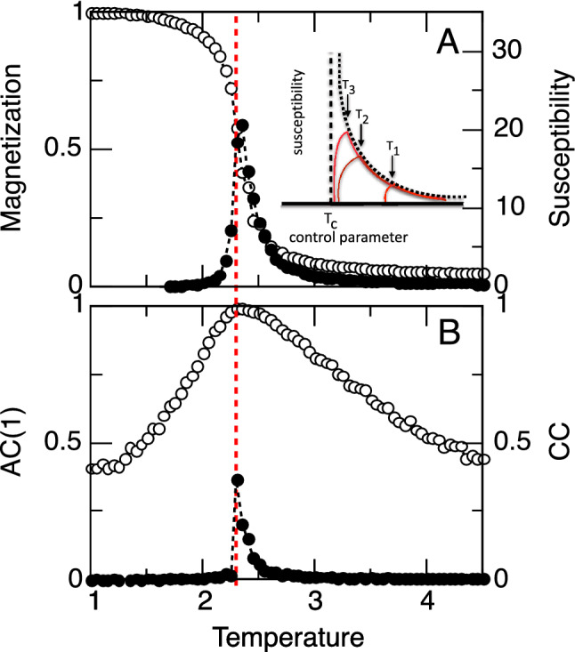
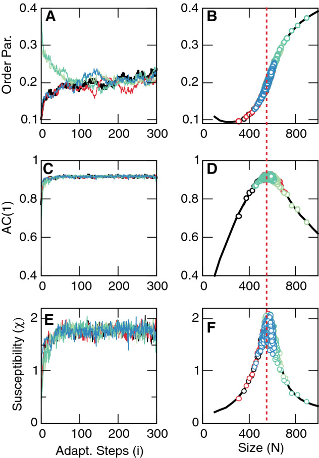
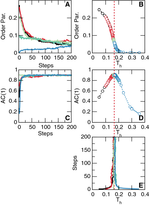
Many complex systems exhibit large fluctuations both across space and over time. These fluctuations have often been linked to the presence of some kind of critical phenomena, where it is well known that the emerging correlation functions in space and time are closely related to each other. Here we test whether the time correlation properties allow systems exhibiting a phase transition to self-tune to their critical point. We describe results in three models: the 2D Ising ferromagnetic model, the 3D Vicsek flocking model and a small-world neuronal network model. We demonstrate that feedback from the autocorrelation function of the order parameter fluctuations shifts the system towards its critical point. Our results rely on universal properties of critical systems and are expected to be relevant to a variety of other settings.

Figure 1

Autocorrelation peaks with susceptibility at $T_c$ in the equilibrium Ising model. Panel A: The order parameter (magnetization; open circles) and susceptibility (filled circles) as function of temperature T. Panel B: Corresponding average pairwise correlation (CC; filled circles) and first autocorrelation coefficient (AC(1); open circles) of the magnetization fluctuations around the instantaneous mean. Dashed vertical line denotes $T_c$. (System size $N={32}^2$, ${10}^4$ MC steps). The inset shows a cartoon of the expected susceptibility as a function of the control parameter for three systems of increasing sizes, where arrows indicate the corresponding optimal points $T_1,T_2,T_3$.

Figure 2

Adaptive control of the Ising model with temperature adjusted iteratively by the autocorrelation of the order parameter. The data illustrate, for a variety of initial temperatures, the convergence of the system to the vicinity of the expected critical temperature $T_c=2.3$. Panels A, C, D, E show, as a function of iteration steps, the first autocorrelation coefficient of the magnetization’ fluctuations, the magnetization, the susceptibility, and the temperature. As seen in Panel C, for any initial temperature the system converges to values near the equilibrium $T_c$ and at the maximum of AC(1) (see panel A). Adaptation parameter $\kappa =0.04$, other parameters as in Fig. 1. Colors denote the evolution of variables toward the critical point starting from five different initial conditions of temperature T: 0.5 (black), 0.1 (red), 0.16 (light green), 0.2 (dark green) and 0.35 (blue).

Figure 3

3D Vicsek model at equilibrium and under adaptive control. Order parameter $\phi$ (Panel A, B), the first autocorrelation coefficient AC(1) of the polarization fluctuations around the mean (Panel C, D) and the susceptibility $\chi$ (Panel E, F) (computed as $\text{var}(\phi )\ast N$) and as a function both of adaptation steps (left columns) and of the system size N (right columns). Notice the overlap between the equilibrium results (solid lines) and the values reached during the adaptive control (open circles) for different initial conditions which converge to the critical size $N_c\sim 560$ denoted by the dashed line. $\eta =0.5$, $v_0=1$, $L=7.5$. $\kappa =800$ and ${10}^4$ MC steps per adaptation iteration step. Colors are used to identify the evolution of the variables toward the critical point, starting from five different initial conditions of size N: 200 (red), 300 (black), 400 (blue), 750 (light green) and 1000 (dark green).

Figure 4

Adaptive control of the neuronal network model. Data corresponds to numerical solutions of the model starting from five different initial conditions of the control parameter $T_h$. Different colors denote the evolution of the variables towards the critical point for each initial condition $T_h$: 0.05 (black), 0.1 (red), 0.16 (light green), 0.2 (dark green) and 0.35 (blue). Nodes threshold $T_h$ are adjusted iteratively according to Eqs. 5–7. Panels A, C and E show the evolution of the order parameter, AC(1) and control parameter $T_h$ respectively. These quantities are plotted against each other in Panels B and D to demonstrate convergence to the critical value of $T_h$ (dashed red line) and to the maximum of AC(1). $\kappa =0.1$ and $5\ast {10}^3$ time steps per adaptation iteration step. Network parameters are: mean degree $<k>=10$, rewiring parameter $\beta =0.3$, system size $N=2^9$. Non null weights chosen from a distribution $p(w)=\lambda e^{-\lambda w}$ with $\lambda =12.5$.

References

1. Bak P. How Nature Works: The Science of Self-organized Criticality. New York: Springer; 1996.
1. Chialvo DR. Emergent complex neural dynamics. Nat. Phys. 2010;6:744. doi: 10.1038/nphys1803. - DOI
1. Mora T, Bialek W. Are biological systems poised at criticality? J. Stat. Phys. 2011;144:268. doi: 10.1007/s10955-011-0229-4. - DOI
1. Honerkamp-Smith AR, Veatch SL, Keller SL. An introduction to critical points for biophysicists; observations of compositional heterogeneity in lipid membranes. Biochim. Biophys. Acta. 2009;1788:53. doi: 10.1016/j.bbamem.2008.09.010. - DOI - PMC - PubMed
1. Beggs JM, Plenz D. Neuronal avalanches in neocortical circuits. J. Neurosci. 2003;23:11167. doi: 10.1523/JNEUROSCI.23-35-11167.2003. - DOI - PMC - PubMed
Publication types