3D mapping and accelerated super-resolution imaging of the human genome using in situ sequencing

Abstract

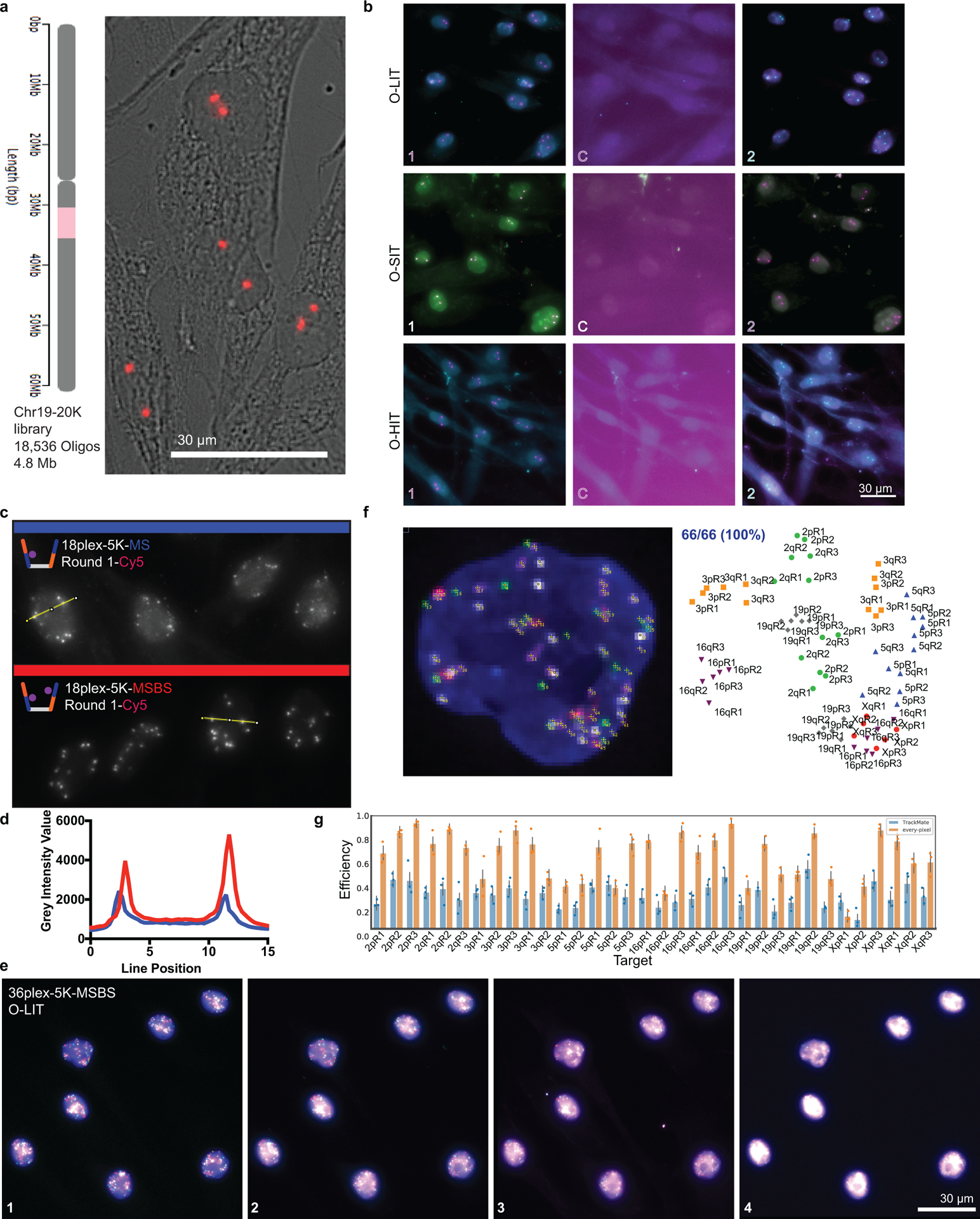
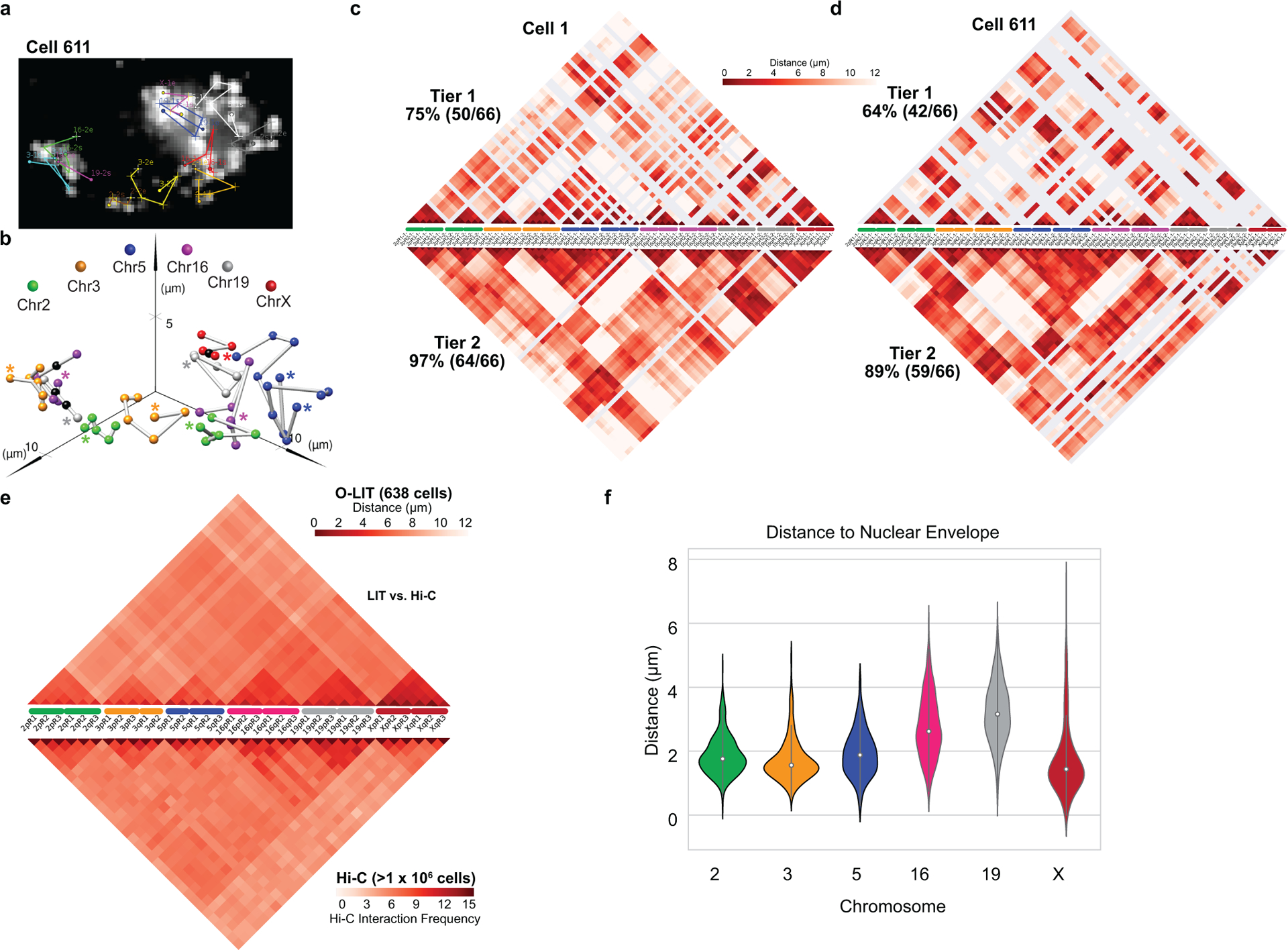
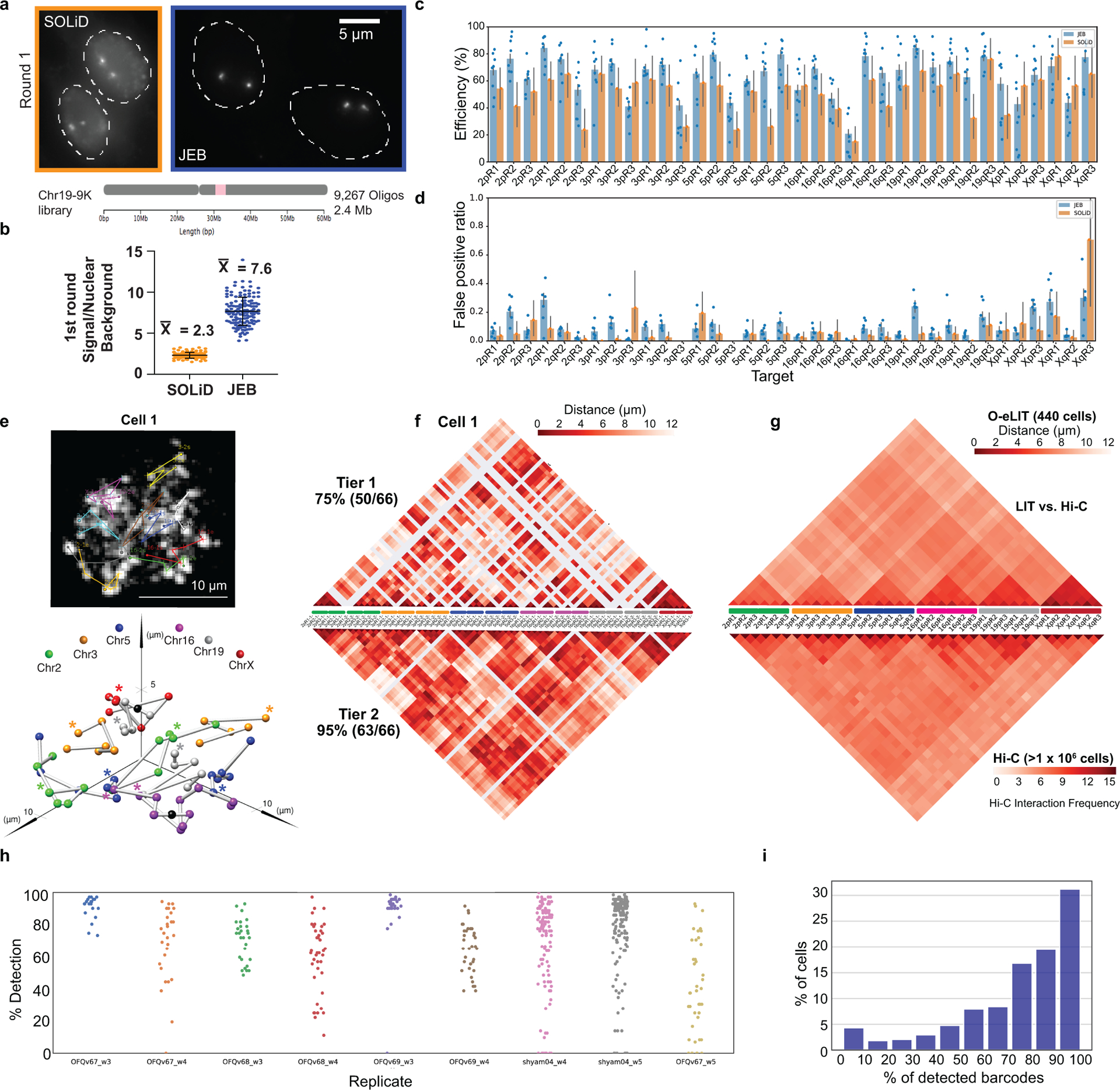
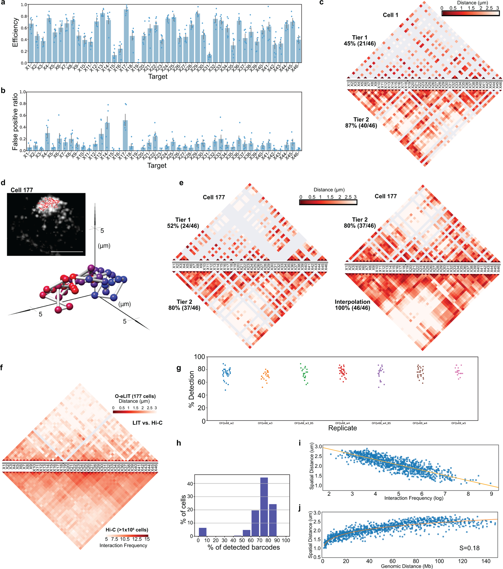
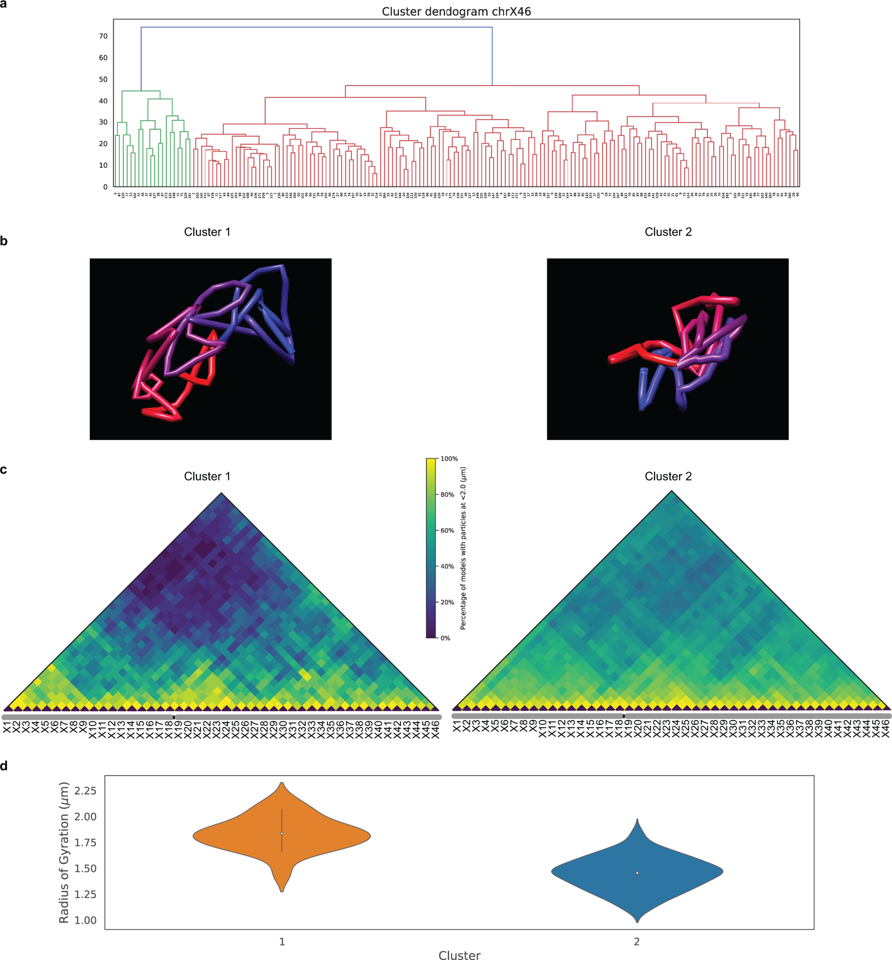
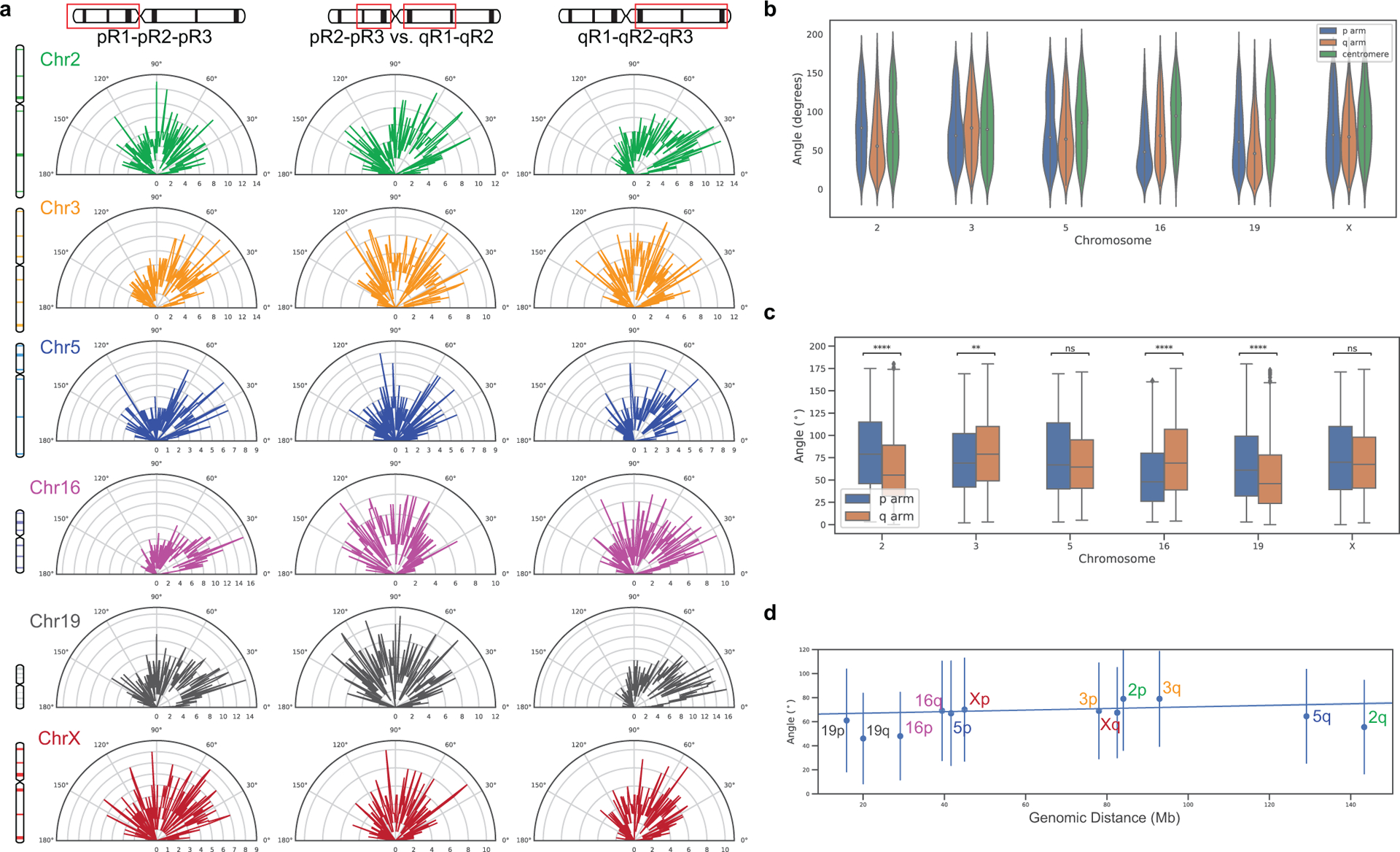
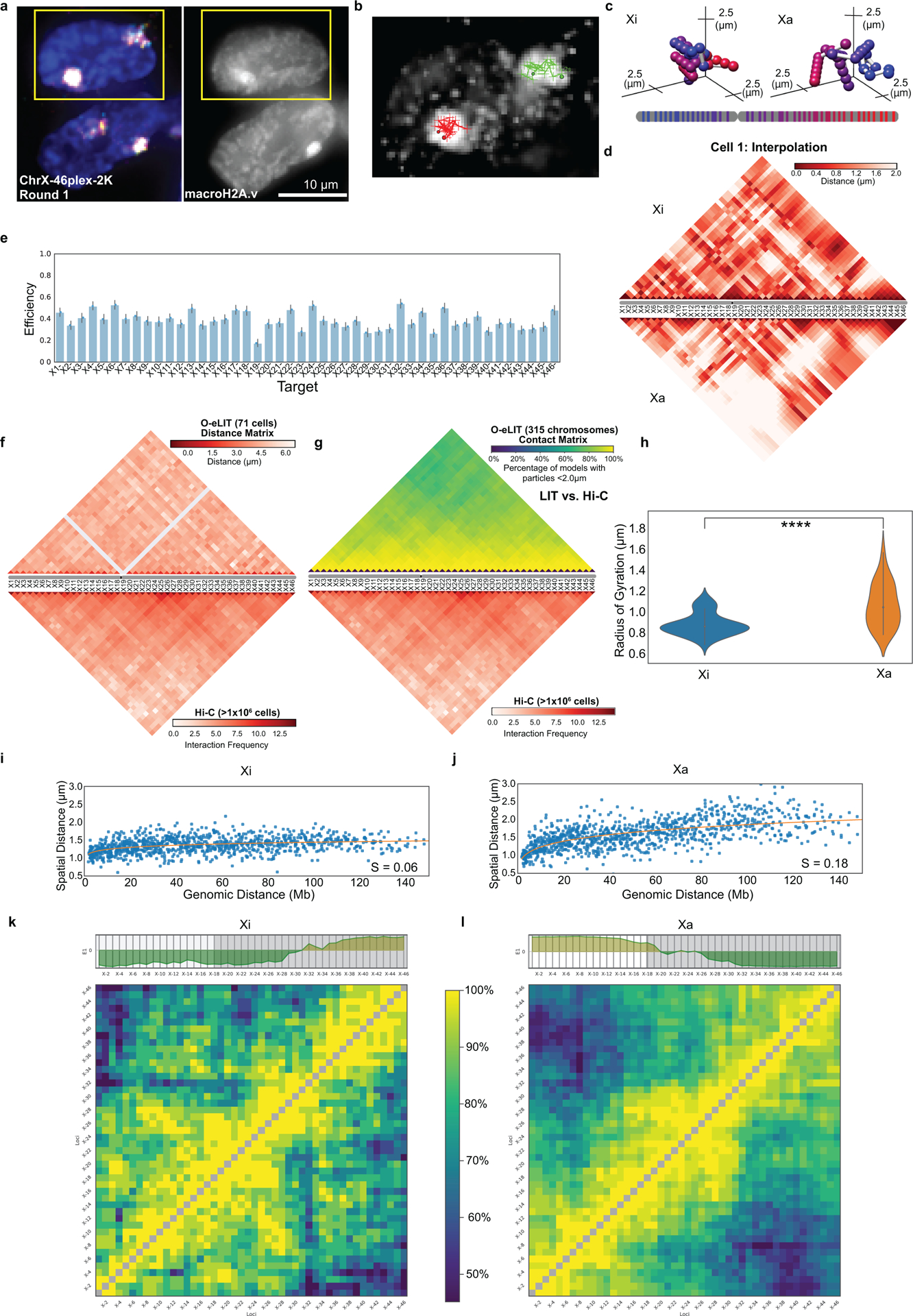
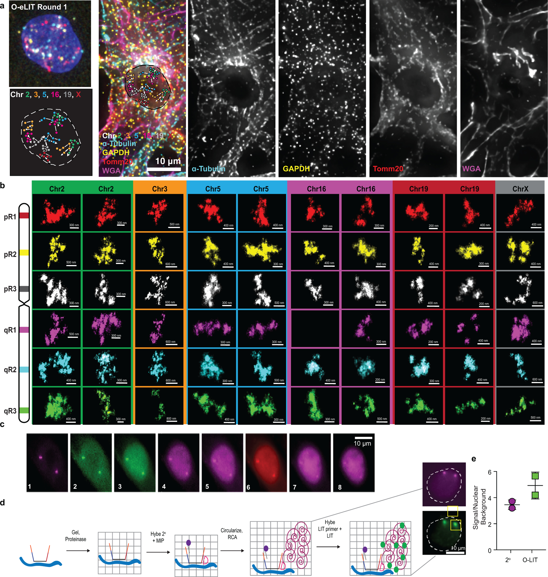
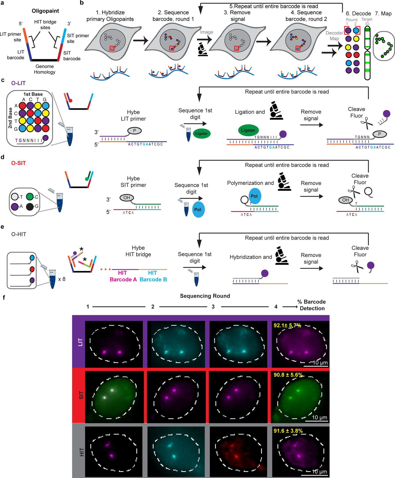
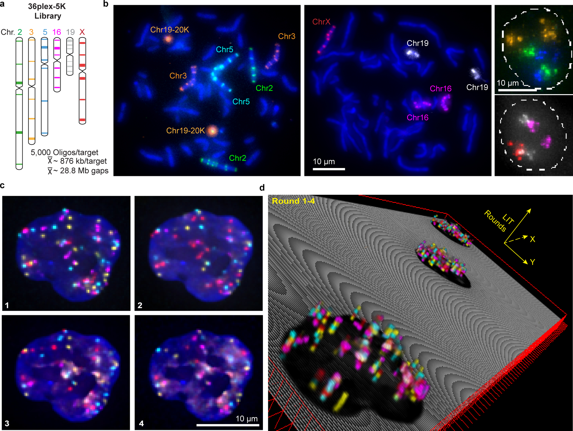
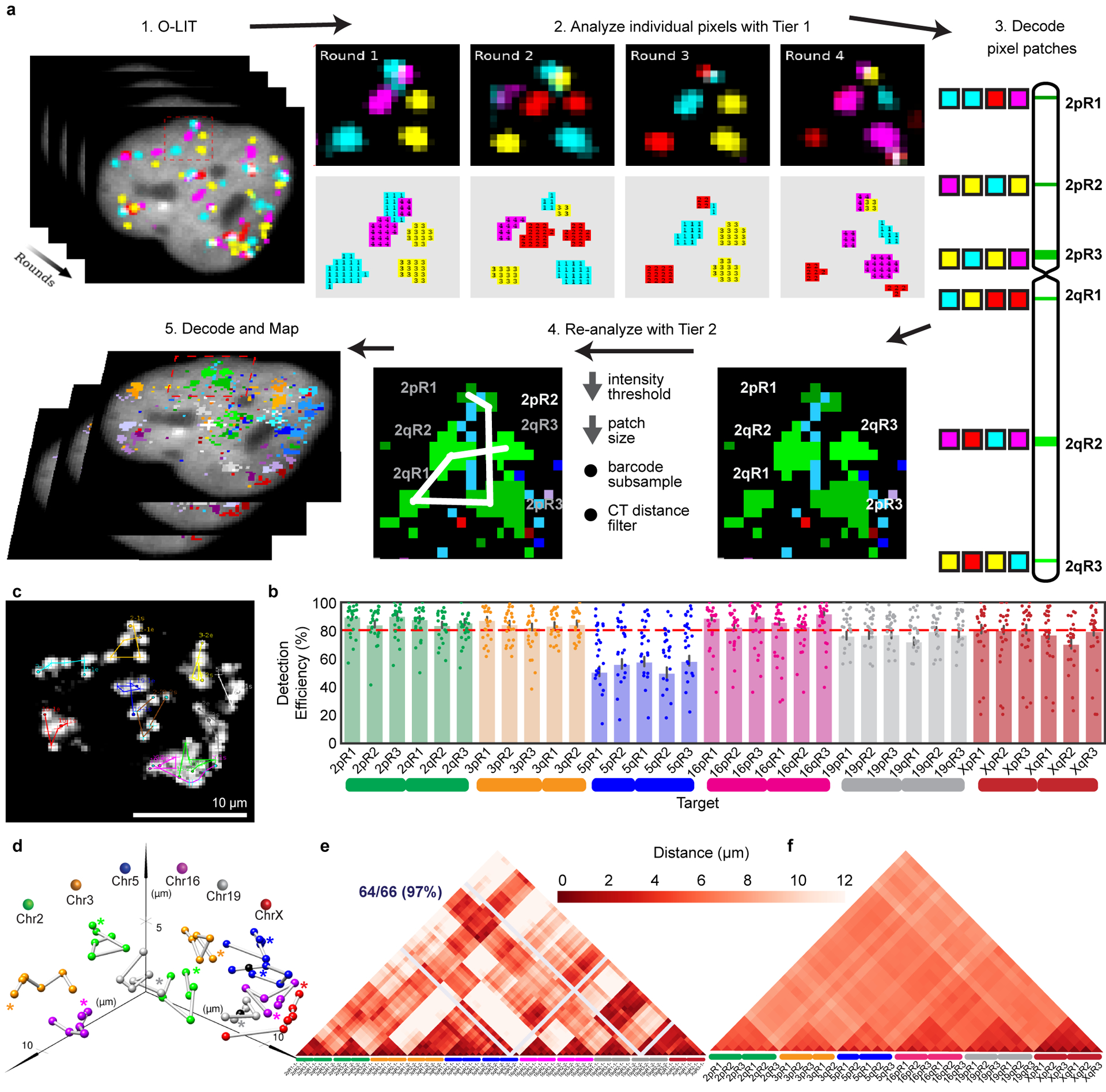
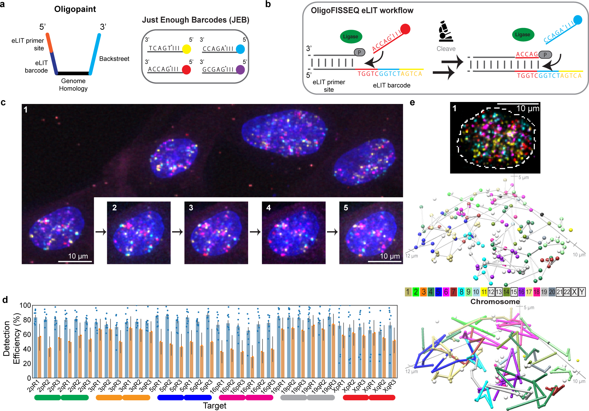
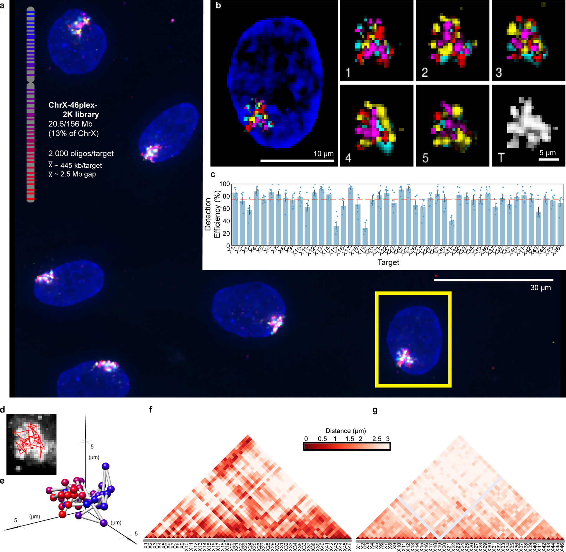
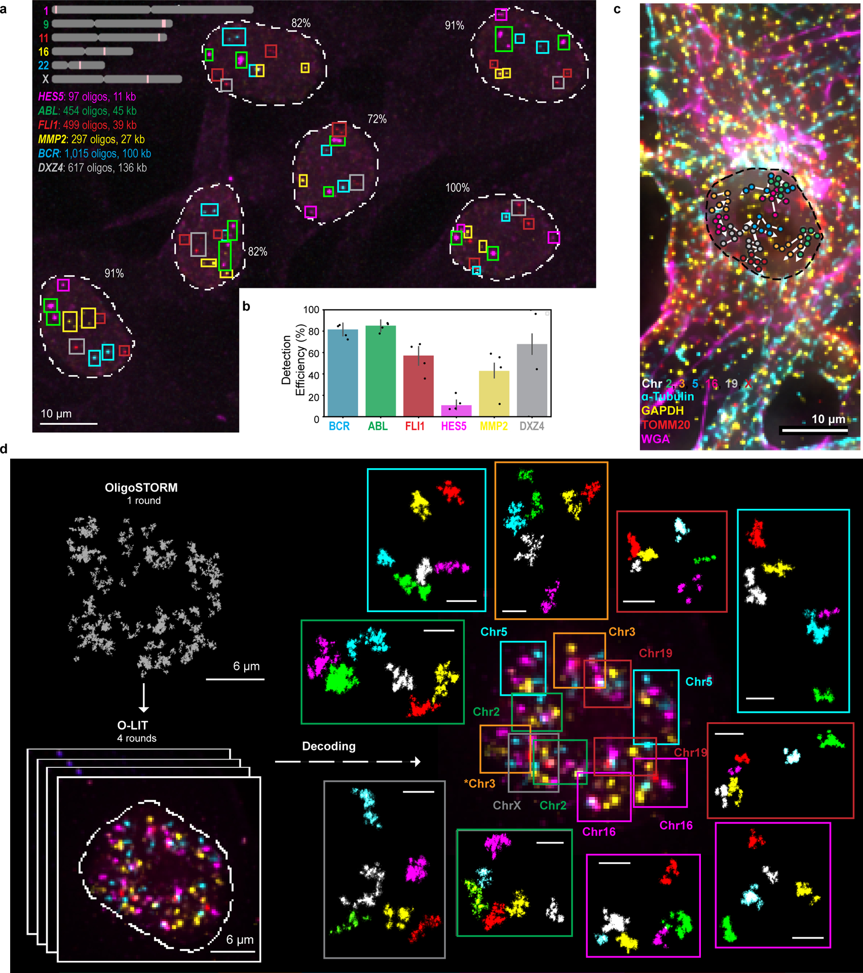
There is a need for methods that can image chromosomes with genome-wide coverage, as well as greater genomic and optical resolution. We introduce OligoFISSEQ, a suite of three methods that leverage fluorescence in situ sequencing (FISSEQ) of barcoded Oligopaint probes to enable the rapid visualization of many targeted genomic regions. Applying OligoFISSEQ to human diploid fibroblast cells, we show how four rounds of sequencing are sufficient to produce 3D maps of 36 genomic targets across six chromosomes in hundreds to thousands of cells, implying a potential to image thousands of targets in only five to eight rounds of sequencing. We also use OligoFISSEQ to trace chromosomes at finer resolution, following the path of the X chromosome through 46 regions, with separate studies showing compatibility of OligoFISSEQ with immunocytochemistry. Finally, we combined OligoFISSEQ with OligoSTORM, laying the foundation for accelerated single-molecule super-resolution imaging of large swaths of, if not entire, human genomes.

Extended Data Fig. 1. Chr19–20K and 36plex-5K-O-LIT optimization

a) Chr19–20K targets 18,536 Oligopaint oligos to human chromosome 19. Right, Chr19–20K detection with secondary oligo (red) in PGP1f cells representative of 5 replicates. b) Signal is completely removed in each OligoFISSEQ method after cleavage. Images showing two rounds of sequencing with a cleavage step (C) and representative of 4 replicates. c) 36plex-5K O-LIT off of both Mainstreet and Backstreet (MSBS; bottom, red) produces stronger signal than off of Mainstreet (MS; top, blue). Cy5 channel from first round of O-LIT. n = 1. d) O-LIT off of both streets produces stronger signal than off of MS. Grey intensity value measurements from yellow lines in panel c. n = 1. e) Raw, non-deconvolved field of view of cell from Figures 2c–d and 3a–c. Maximum z-projection. n = 1. f) Manual decoding of cell from panel c and Figures 2c–d and 3a–c yields 100% target recovery. n = 1. g) Tier 1 detection efficiency after 36plex-5K O-LIT off of both streets and detected with TrackMate (blue, 29.93 ± 4.9%) or Every-pixel (orange, 62.8% ± 4.8%). n = 111 cells from 3 replicates. Detection efficiency from individual replicates are plotted. Error bars represent 95% bootstrap confidence interval of the mean.

Extended Data Fig. 2. Detection efficiency after 36plex-5K O-LIT

a) Detection efficiency without filtering after 36plex-5K O-LIT off of both streets. 95 ± 5.15% of targets are detected (n = 611 from 15 replicates). Detection efficiency from individual replicates are plotted. Error bars represent 95% bootstrap confidence interval of the mean. b) False positive (FP) discovery rate from panel a. FP discovery rate from individual replicates are plotted. Error bars represent 95% bootstrap confidence interval of the mean. c) Tier 1 detection efficiency after 36plex-5K O-LIT off of Mainstreet (orange, 61.93 ± 12%, n = 53 from 2 replicates) versus off of both streets (blue, 62.17% ± 6.68%, n = 611 cells from 15 replicates). Detection efficiency from individual replicates are plotted. Error bars represent 95% bootstrap confidence interval of the mean. d) FP discovery rate from panel c. Using Mainstreet = 8.64% and using both streets = 5.29%. FP discovery rate from individual replicates are plotted. Error bars represent 95% bootstrap confidence interval of the mean. e) Tier 2 detection efficiency after 36plex-5K off of Mainstreet (orange, 92.3% ± 3.42% from 53 cells from 2 replicates) versus off of both streets (blue, 80.19 ± 7.29%, n = 611 cells from 15 replicates). Detection efficiency from individual replicates are plotted. Error bars represent 95% bootstrap confidence interval of the mean. f) Detection efficiency after 36plex-5K O-LIT off of both streets for individual cells from 15 replicates in panel e. g) Percentage of cells displaying a range of efficiencies of barcode detection after 36plex-5K O-LIT off of both streets. Data taken from panel e. h) Principal component analysis showing lack of batch effect in 36plex datasets (n = 1171 cells from 15 36plex-5K O-LIT replicates and 8 36plex-1K O-eLIT replicates).

Extended Data Fig. 3. O-LIT with 36plex-5K to interrogate genome organization

a) Chromosome traces of Cell 611 after Tier 2 detection of cell 611 after four rounds of O-LIT 36plex-5K off of both streets. 59/66 (89%) of 36plex-5K targets were detected. Image is from the first round of O-LIT with target identities. n = 1. b) Ball and stick of Cell 611. Colored spheres represent chromosomal targets, while black spheres represent targets that were not detected and, thus, were placed by calculating the median proportionate distance between flanking detected targets. Beginning of chromosome (e.g. 2pR1) marked by an asterisk. c) Single-cell pairwise spatial distance matrix after Tier 1 (top) and Tier 2 (bottom) detection of the nucleus in Figure 3. Targets are represented on the x-axis with homologs separately displayed. Undetected targets are represented by grey lines. d) Single-cell pairwise spatial distance matrix after Tier 1 (top) and Tier 2 (bottom) detection of Cell 611. Targets are represented on the x-axis with homologs separately displayed. Undetected targets are represented by grey lines. e) 36plex-5K population pairwise spatial distances (top, from Fig. 3f). Average pairwise spatial distances from cell population after Tier 1 detection (n = 611 from 15 replicates). (Spearman’s rank correlation 0.705, two-sided p-value for a hypothesis test whose null hypothesis is that two sets of data are uncorrelated = 1.77e-174). Measurements from homologous targets were combined. Bottom, Hi-C data of 36plex-5K targets obtained from (Nir et al. 2018). f) Average distances between the nuclear membrane and the closest of the six targets imaged for each chromosome. (n = 686, 668, 364, 586, 760, and 494 for Chr2, 3, 5, 16, 19, and X, respectively.) The thick line in each violin plot represents the Interquartile range (IQR), the white dot marks the median and the thin lines extend 1.5 times the IQR.

Extended Data Fig. 4. O-LIT with 36plex-5K to interrogate homolog organization

a) Minimum distances between heterologous and homologous chromosomes. All measurements represent distances between the geometric centers of chromosomes for which all six targets were imaged. Distances between a chromosome and a heterologous chromosome is the shorter of the two distances between that chromosome and the two homologous copies of the heterologous chromosome (n = 686, 668, 364, 586, 760, and 494 for Chr2, 3, 5, 16, 19, and X, respectively). Inter-homolog distances for Chr16 and 19 are less than those for Chr2, 3, and 5 (independent-samples t-test p = 4.28 × 10–37). Boxes represent the IQR (25th, 50th and 75th percentiles) and whiskers extend 1.5 times the IQR b) Number of cells with varying numbers of homologs split by K-means clustering. The K-means algorithm was applied to 258 nuclei, individually, to cluster chromosomes into two groups based on proximity and then report the number of homolog pairs that were split by the clustering. A value of “5” indicates that the homologs from each five pairs of imaged autosomes in a single nucleus clustered into two spatially separate groups. Observed, PGP1f cells. Directed random, raw positions in Observed but with the chromosome identities of all positions randomized, with the larger chromosomes (2, 3, 5) biased towards the nuclear periphery and smaller chromosomes (16 and 19) biased towards the nuclear interior. Completely random category, randomization of the chromosome identities carried out with no spatial bias. The significance of each pair was evaluated from a two proportion z-test with n=258 for each category with a null hypothesis of equal proportion and a significance level of 0.05. c) Density plots of homolog positions. Built by using Kernel density estimation (KDE) of nuclei projected and aligned along the x-y plane of the position of the chromosomes. d) Pie charts of total number of cells with homologs split by a virtual line along the y-axis. e) Number of aligned cells with homologs split by a virtual line parallel to the y-axis at different distances from the origin, that is, number of autosomes with one of their homologs on the left of the line and the other on the right (n = 258 for each category). Boxes represent the IQR (25th, 50th and 75th percentiles) and whiskers extend 1.5 times the IQR.

Extended Data Fig. 5. O-eLIT with JEB

a) Chr19–9K. One round of O-LIT (SOLiD) or O-eLIT (JEB) off of Mainstreet. Maximum z-projections representative of 2 replicates. b) Chr19–9K signal over nuclear background measurements after one round of O-LIT (orange; n = 113 puncta from 55 cells from 2 replicates) or O-eLIT (blue; n = 136 puncta from 57 cells from 2 replicates). Bar is the mean and SD. c) Tier 1 detection of 36plex-1K after five rounds of O-LIT with SOLiD reagents (orange; average of 51.75%, n = 41) or O-eLIT with JEB (blue; average of 61.2 ± 10.2%, n = 440 from 9 replicates). Detection efficiency from individual replicates are plotted. Error bars represent 95% bootstrap confidence interval of the mean. 36plex-1K library shares first 1,000 Oligopaint oligos of each target in 36plex-5K. For example, for target 2pR1, 36plex-5K spans the chromosomal region from nt position 1,002,895 to 1,660,898 (~658 kb), whereas 36plex-1K spans the region from nt 1,002,895 to 1,147,495 (~144 kb). d) FP discovery rate from panel c. SOLiD = 7.49% and JEB = 8.95%. FP discovery rate from individual replicates are plotted. Error bars represent 95% bootstrap confidence interval of the mean. e) Chromosome traces and ball and stick of Fig. 4c cell after Tier 2 detection and five rounds of O-eLIT 36plex-1K. 63/66 (95%) targets were detected. Asterisks, beginning of chromosomes. n = 1. f) Single-cell pairwise spatial distance matrices of panel C cell. g) 36plex-1K population pairwise spatial distance measurements (top, from Fig. 3f). Average pairwise spatial distance from cell population after Tier 1 detection (n = 440 from 9 replicates). Measurements from homologous targets were combined. Bottom, Hi-C data of 36plex-5K targets obtained from (Nir et al. 2018). h) 36plex-1K detection rate for individual cells from 9 replicates. i) Percentage of cells displaying a range of efficiencies of barcode detection after 36plex-1K O-eLIT off of Mainstreet.

Extended Data Fig. 6. O-eLIT with ChrX-46plex-2K

a) ChrX-46plex-2K O-eLIT Tier 1 detection off of one street and off of both streets combined (52.86 ± 5.78% from 177 cells from 7 replicates). Detection efficiency from individual replicates are plotted. Error bars represent 95% bootstrap confidence interval of the mean. b) FP discovery rate from panel a. Error bars represent 95% bootstrap confidence interval of the mean. c) Single-cell pairwise spatial distance matrix after Tier 1 (top) and Tier 2 (bottom) detection of Cell 1 from Figure 5b. Undetected targets are represented by grey lines. d) Chromosome traces (top) and ball and stick representation (bottom) of Cell 177 after Tier 2 detection and interpolation and five rounds of O-eLIT on ChrX-46plex-2K off of both streets. Image is from the first round of O-eLIT with target identities. n = 1. e) Single-cell pairwise spatial distance matrix after Tier 1 (top), Tier 2 (bottom) of Cell 177 (left), and Tier 2 (top) and interpolation (bottom) of same cell (right). Undetected targets are represented by grey lines. f) ChrX-46plex-2K population pairwise spatial distances (top). Average pairwise spatial distances from cell population after Tier 1 detection (n = 177 from 7 replicates). Bottom, Hi-C (Nir et al. 2018) data of ChrX-46plex-2K targets. (Spearman’s rank correlation 0.641, two-sided p-value for a hypothesis test whose null hypothesis is that two sets of data are uncorrelated = 7.074e-245). g) ChrX-46plex-2K detection rate for individual cells from 7 replicates. h) Percentage of cells displaying a range of efficiencies of barcode detection after ChrX-46plex-2K O-eLIT. i) Mean spatial distance versus Interaction frequency of Hi-C (Nir et al. 2018) of ChrX-46plex-2K targets. Pearson correlation coefficient (r = −0.84) and p-value = 5.08E-275 (two-sided, using slope = 0 for null hypothesis and Wald Test with t-distribution as test statistic) of the linear least-squares regression. j) Mean spatial distance versus genomic distance for all pairwise ChrX-46plex-2K targets (n = 177 from 7 replicates).

Extended Data Fig. 7.. O-eLIT identifies clusters after ChrX-46plex O-eLIT

a) Hierarchical clustering based on structure of ChrX traces from ChrX-46plex after 5 rounds of O-eLIT and Tier 2 detection yielded two clusters (Cluster 1 = 20; Cluster 2 = 156). See Methods for more details. b) ChrX representative models (existing traces that are closer to the virtual centroid) of the two clusters obtained after Hierarchical clustering in panel a. c) ChrX-46plex-2K population contact matrix of two clusters derived after Hierarchical clustering in panel a where pairwise spatial distances are considered to be in contact if less than 2 μm apart. d) Radius of gyration for the two clusters (Cluster 1 = 20; Cluster 2 = 156) derived after the hierarchical clustering shown in panel a. The thick line in each violin plot represents the Interquartile range (IQR), the white dot marks the median and the thin lines extend 1.5 times the IQR.

Extended Data Fig. 8. Angles from 36plex

a) Measurements of angles formed by three points along the p arm (left), q arm (right), and intersection of vectors formed by pR2-pR3 and qR1-qR2 (middle) for each chromosome. Measurements were obtained by combining data from 36plex-5K and 36plex-1K analyses and selecting chromosomes that had all six targets identified. Chr2: n = 686, Chr3: n = 668, Chr5: n = 363, Chr16: n = 586, Chr19: n = 760, ChrX: n = 493 (n = 1,051 cells from 24 replicates; for 36plex-5K, n = 611 from 15 replicates; for 36plex-1K, n = 440 from 9 replicates). b) Distribution of angles formed by segments in panel a. The thick line in each violin plot represents the Interquartile range (IQR), the white dot marks the median and the thin lines extend 1.5 times the IQR. c) Box plots comparing p and q arm angles. Two-sided student’s t-test with null hypothesis of equal mean was performed to compare arms, ns p > 0.05, * p ≤ 0.05, ** p ≤ 0.01, *** p ≤ 0.001, **** p ≤ 0.0001. Boxes represent the IQR (25th, 50th and 75th percentiles) and whiskers extend 1.5 times the IQR. Sample size information in a). Exact p-values for each chromosome: Chr.2 = 4.149e-16, Chr.3 = 0.004, Chr.5 = 0.093, Chr.16 = 1.357e-14, Chr.19 = 3.325e-11, Chr.X = 0.101. d) Linear least-squares regression between arm angle and arm length with Pearson correlation coefficient r = 0.26 and p-value = 0.42 (two-sided, using slope = 0 for null hypothesis and Wald Test with t-distribution as test statistic).

Extended Data Fig. 9. O-eLIT comparison of X chromosomes in female IMR-90 cells after ChrX-46plex-2K O-eLIT off of both streets

a) First round of O-eLIT sequencing. MacroH2A.1 immunostaining after five rounds of O-eLIT marks the Xi. n = 1. b-c) Xi and Xa traces (b) and ball and stick (c) of panel a nucleus after Tier 2 analysis and interpolation of missing targets. Sphere color corresponds to chromosome cartoon. n = 1. d) Single-cell pairwise spatial distances after interpolation of missing targets in panel a. e) Tier 2 target detection efficiency after five rounds of O-eLIT. 38.57% of targets are detected in 71 cells. Detection efficiency from individual replicates are plotted. Error bars represent 95% bootstrap confidence interval of the mean. f) Population pairwise spatial distances after Tier 1 detection (n = 71 cells) and Hi-C data of IMR-90 cells (Rao et al. 2014). g) Population contact maps (top) where two targets are considered to be in contact if less than 2 μm apart (n = 315 chromosomes). Bottom, Hi-C data as in panel f. (Spearman’s rank correlation with the Hi-C matrix is r =0.733, two-sided p-value for a hypothesis test whose null hypothesis is that two sets of data are uncorrelated = 2.564 × 10e-175). h) Radius of gyration for the Xi (n = 40 chromosomes) and Xa (n = 31 chromosomes). The thick line in each violin plot represents the Interquartile range (IQR), the white dot marks the median and the thin lines extend 1.5 times the IQR. P-value = 7.08 × 10e-6 (two-sided t-test whose null hypothesis is equal means). i-j) Linear plot of the mean spatial distance versus the genomic distance for all pairwise targets for Xi (n = 40 chromosomes) and Xa (n = 31 chromosomes). k-l) Population contact maps for Xi (n = 40 chromosomes) and Xa (n = 31 chromosomes) with eigenvector analysis used to identify different domains. X1-X18 (white) and X19-X46 (grey) targets p and q arms, respectively.

Extended Data Fig. 10. OligoFISSEQ applications

a) O-eLIT and immunofluorescence (IF). 36plex-1K was sequenced 5 rounds with O-eLIT off Mainstreet. Then, the same sample was prepared for IF and stained with antibodies. Samples were counterstained with wheat germ agglutinin (WGA) to stain membranes. Images are from deconvolved, maximum z-projections representative of 2 replicates. b) Chromosomal regions imaged with OligoSTORM from Fig. 6d enlarged and displayed separately. Orientation may differ from Fig. 6d. n = 1. c) 8 rounds of O-LIT sequencing of Chr19–9K off of Mainstreet. Images are maximum z-projections. Signal is detectable in all rounds even though the imaging was conducted without the advantage of eLIT, suggesting that 8 rounds of O-eLIT will produce even stronger signals. Images are representative of 2 replicates. d) O-LIT is compatible with gel embedding and target amplification via rolling circle amplification (RCA). Chr19–9K was hybridized to PGP1f cells, after which the sample was embedded in a hydrogel and then cleared of cellular background with proteinase. Next, a molecular inversion probe (MIP) was hybridized to a Chr19–9K specific barcode on Backstreet as well as a fluorophore labeled (purple) secondary oligo to Mainstreet to visualize Chr19–9K Oligopaint oligos. MIPs were circularized via ligation and RCA, after which the first digit of the barcode was sequenced using O-LIT (green). Images representative of 2 replicates. e) Comparison of secondary fluorophore signal (2°) versus first round sequencing signal (LIT) from puncta in panel b images. Center values are mean values (3.4 for 2° and 4.9 for O-LIT) with SD.

Fig. 1.. OligoFISSEQ

a) Oligopaint oligo used for OligoFISSEQ. Portions of the LIT and SIT primer sites and barcodes can function as binding sites for HIT bridges (panel e) as well as priming sites to amplify the Oligopaint library. LIT primers and barcodes can be encoded on both streets to increase signal. Some libraries used reverse priming sites that were chromosome-specific (common to oligos targeting the same chromosome). b) General OligoFISSEQ workflow. In step 7, mapped targets correspond to Target ID text color in step 6 and chromosome cartoon. c) O-LIT. After the phosphorylated LIT primer (P) is hybridized, it is ligated to an 8-mer (TGNNNIII), the first two nts of which correspond to a specific fluorophore; as Oligopaint barcodes are pre-defined, each fluorophore corresponds to only a single barcode digit. N denotes a mixture of A, C, T, or G, and I denotes deoxyinosine, a universal base. d) O-SIT. SIT primers contain 3’hydroxyls (OH). A and C are conjugated to distinct fluorophores (shown here as purple and green, respectively), T to two fluorophores (grey), with G remaining unlabeled (black). e) O-HIT. In this iteration using three fluorophores and 6 barcodes, each round of hybridization uses three fluorophore-labeled oligos, and two rounds suffice to identify which barcode resides at a barcode position. Given 4 barcode positions, HIT is completed within 8 rounds of hybridization. *, two bridge oligos bringing in a total of 4 HIT barcodes. f) Representative images after 4 rounds of O-LIT, O-SIT, and O-HIT using Chr19–20K on PGP1f cells. Images represent maximum intensity z-projections. The first round of SIT identifies deoxyadenosine (labeled by a combination of purple and green and thus appears white). Mean barcode detection efficiencies with SD for LIT, SIT, and HIT represent 85, 66, and 79 total cells, respectively, from 4 replicates.

Fig. 2.. OligoFISSEQ-LIT on 36plex-5K

a) Targets of the library. Chromosome number color-coded to correspond to images in panel b. Each target corresponds to a unique barcode. b) Metaphase chromosome spreads of male lymphoblast cells (left; cells from Applied Genetics; Methods) and interphase nuclei from PGP1f cells (right) representative of four replicates. All six targets on any single chromosome were labeled with secondary oligos carrying the same species (color) of fluorophore. Chr19–20K was used as a positive control in metaphase chromosome spreads. Maximum z-projections. c) Four rounds of O-LIT off of both streets of 36plex-5K. Images are from deconvolved, five-color merged maximum z-projections. n = 1. d) 3D representation of a field of view (FOV) containing three cells sequenced with four rounds of O-LIT. Sequencing rounds are represented on the z-axis, with the first being closest to the DAPI-determined nuclear outline (black). Maximum z-projection of sequencing signal from each round was taken, duplicated (2-images total for better visualization), and then stacked on top of each other. The lower left cell corresponds to the cell in panel c.

Fig. 3.. Every-pixel analysis pipeline on 36plex-5K

a) Analysis pipeline. Sequencing rounds (Step 1) are analyzed at the level of individual pixels using Tier 1 parameters with thresholds for signal intensity and pixel patch size (Step 2) and then decoded (Step 3). Missing targets and false positives are filtered by re-analyzing images with Tier 2 parameters (Step 4) to produce traces (Step 5). Tier 2 decreases thresholds for signal intensity and pixel patch size, subsamples barcodes, and applies filters for chromosome territories. 1 = FITC, 2 = Cy3, 3 = TxRed, 4 = Cy5. b) 36plex-5K Tier 2 detection efficiency after sequencing off of both streets. 80.2 ± 7.3% of targets are detected in 611 cells from 15 replicates. X-axis, chromosomal targets. Detection efficiency from individual replicates are plotted. Dashed red line marks the mean over all chromosomal targets. 3qR3 and 5pR3 share a barcode and are not included (see text). For unknown reasons, Chr5 target detection was less robust. Error bars represent 95% bootstrap confidence interval of the mean. c) Chromosome traces of Figure 2c nucleus after Tier 2. 64/66 (97%) of targets were detected. N = 1. d) Ball and stick traces of panel b nucleus. Colored spheres represent targets; black spheres represent undetected targets and, thus, positioned by calculating the median proportionate distance between flanking detected spheres. Grey lines between signals, extrapolations. Asterisks, beginning of chromosomes. e) Single-cell pairwise spatial distance matrix after Tier 2 detection of panel b nucleus. Homologs separately displayed. Centroids of targets were used for this and all subsequent spatial distance matrices. Grey lines, undetected targets. f) 36plex-5K population pairwise spatial distance measurements after Tier 1 detection (n = 611 from 15 replicates). Homologous target measurements were combined. Overall greater distances of Chr2, Chr3, Chr5, and X may reflect more peripheral positioning, while lesser distances of Chr16 and Chr19 may reflect more central positioning.

Fig. 4.. OligoFISSEQ-eLIT

a) JEB technology reduces the pool of labeled 8-mers to four. Left, design of Oligopaint oligos in libraries, such as 36plex-1K, that use eLIT. Right, JEB labeled 8-mers complementary to the 5-nt eLIT barcode digit. I, universal base, deoxyinosine. While eLIT is compatible with a variety of barcode configurations, our current application uses barcodes consisting of 5 digits each, wherein each digit is one of only four distinct 5-nt sequences. To further reduce the complexity of the pool of 8-nt oligos, we also use the universal base, deoxyinosine in positions 6, 7, and 8. In short, JEB reduces the pool of labeled oligos from 1,024 to 4 (Extended Data Fig. 5a–b). b) eLIT workflow with JEB. See legend to Figure 1c for details. c) Five rounds of sequencing with O-eLIT. Left, PGP1f cells after first round of sequencing. Right, images from five rounds of sequencing (1–5) of one nucleus from panel c (yellow square); T, totality of targets labeled simultaneously with a secondary oligo complementary to a barcode present on each oligo. Extranuclear puncta are fiducial tetraspeck beads (Thermo Fisher). Images are deconvolved maximum z-projections. n = 1. d) Tier 2 target detection efficiency of 36plex-1K after five rounds of O-LIT with SOLiD reagents (orange; average of 54.6%; n = 41) or O-eLIT with JEB (blue; average of 74 ± 11.2%; n = 440 from 9 replicates). Detection efficiency from individual replicates are plotted. Error bars represent 95% bootstrap confidence interval of the mean. e) First O-eLIT round of 129-plex (top; deconvolved maximum-intensity z projection; n = 1). Tier 2 tracings (middle; white spheres are tier 1 duplicated barcodes that did not move to tier 2, with untraced chromosomes boxed in color key). Sticks color-coded to facilitate visualization (bottom). Oligonucleotide target density was 5.8 to 11.9 per kb.

Fig. 5.. Tracing 46 regions along Chromosome X

a) Targets of ChrX-46plex-2K and nuclei after a first round of O-eLIT sequencing off of both streets in PGP1f. Images are from deconvolved maximum intensity z-projection. n = 1. b) Five rounds of sequencing with O-eLIT off of both streets. Nucleus from panel a (yellow square). Left, view of DAPI stained nucleus after first round of sequencing. White numbers, round of sequencing. T, totality of targets labeled simultaneously with a secondary oligo complementary to a barcode present on all oligos. Images are from deconvolved maximum z-projection. n = 1. c) Tier 2 target detection efficiency after five rounds of O-eLIT off of both streets in PGP1f cells. The mean detection efficiency marked by the red dashed line was 74.29 ± 2.5% (n = 177 from 7 replicates), averaging detection efficiencies off of one street (73.7 ± 2.97%, n = 122 from 5 replicates) and off of both streets (75.3 ± 1.97%, n = 55 from 2 replicates). Particularly difficult was X19, being detectable only 0% and 28% of the time after Tier 1 (Extended Data Fig. 6a) and Tier 2, respectively Detection efficiency from individual replicates are plotted. Error bars represent 95% bootstrap confidence interval of the mean. d-e) Chromosome traces (d) and 3D visualization (e) of the nucleus in Figure 5b after Tier 2 analysis and interpolation of missing targets. Sphere color corresponds to chromosome cartoon in panel a. n = 1. f) Single-cell pairwise spatial distances after interpolation of missing targets of nucleus in panel b. g) Population pairwise spatial distances (n = 177 from 7 replicates) after Tier 1 detection (combining reads off of Mainstreet with reads off of both streets).

Fig. 6.. OligoFISSEQ extensions and applications

a) O-eLIT detection of single gene targets after sequencing off of both streets. Colored squares mark gene targets identified after 5 rounds of sequencing. Number reflects percentage of targets detected out of 11 (5 autosomal genes x 2 in addition to DXZ4 on the X). Image from deconvolved maximum intensity z-projection and representative of 2 replicates. b) Tier 1 target detection efficiency from experiment in panel a (n = 61 from 2 replicates). Tier 2 inapplicable due to lack of targets from the same chromosome. Detection efficiency from individual replicates are plotted. Error bars represent 95% bootstrap confidence interval of the mean. c) Combining O-LIT and immunofluorescence. 36plex-5K was sequenced for four rounds with O-LIT off of both streets, followed by immunofluorescence and staining with wheat germ agglutinin (WGA). Image from deconvolved maximum intensity z projection with chromosome traces overlaid. n = 1. d) 36plex-5K was hybridized to PGP1f cells and imaged with 1 round of OligoSTORM (2 hours) to visualize all 66 targets simultaneously, followed by 4 rounds of O-LIT (2 – 3 hours per round) to decode targets. Top left, OligoSTORM image showing entire field of view with all unidentified targets. Bottom left, micrograph from first round of O-LIT; image from deconvolved maximum z-projection. Right, all 6 chromosomes identified (central image decorated with colored squares, color coded by chromosome as shown) and then arrayed, in super-resolution, around the central nucleus. All 66 targets excepting one region on Chr16, were detected and identified by O-LIT, with one homolog of Chr3 (*) not captured by OligoSTORM because it happened to fall outside the field of view. All scale bars for OligoSTORM images, 1 μm. e) Each chromosomal region imaged with OligoSTORM from panel d is displayed separately; orientation may differ from that in panel e. n = 1.

References

1. Hu Q, Maurais EG & Ly P Cellular and genomic approaches for exploring structural chromosomal rearrangements. Chromosome Res 28, 19–30 (2020). - PMC - PubMed
1. Bolzer A et al. Three-Dimensional Maps of All Chromosomes in Human Male Fibroblast Nuclei and Prometaphase Rosettes. PLoS Biology 3, e157 (2005). - PMC - PubMed
1. Cremer T & Cremer M Chromosome territories. vol. 2 (2010). - PMC - PubMed
1. Beliveau BJ et al. Versatile design and synthesis platform for visualizing genomes with Oligopaint FISH probes. Proceedings of the National Academy of Sciences 109, 21301–21306 (2012). - PMC - PubMed
1. Beliveau BJ et al. Single-molecule super-resolution imaging of chromosomes and in situ haplotype visualization using Oligopaint FISH probes. Nature Communications 6, 7147 (2015). - PMC - PubMed
Publication types