Constrained sampling from deep generative image models reveals mechanisms of human target detection

Abstract

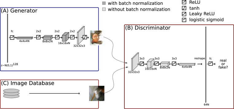
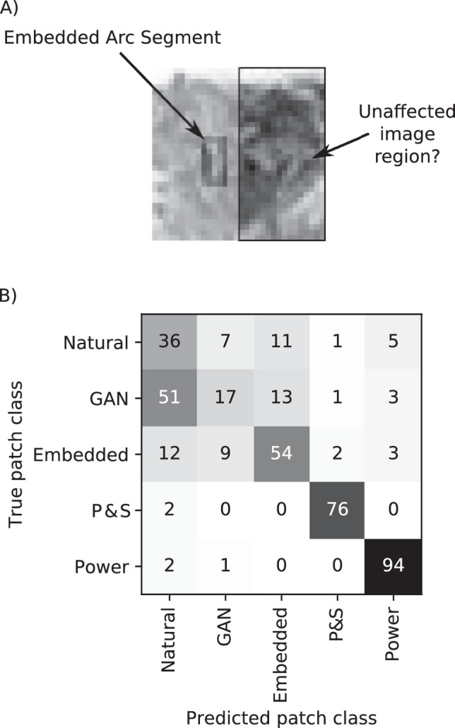
The first steps of visual processing are often described as a bank of oriented filters followed by divisive normalization. This approach has been tremendously successful at predicting contrast thresholds in simple visual displays. However, it is unclear to what extent this kind of architecture also supports processing in more complex visual tasks performed in naturally looking images. We used a deep generative image model to embed arc segments with different curvatures in naturalistic images. These images contain the target as part of the image scene, resulting in considerable appearance variation of target as well as background. Three observers localized arc targets in these images, with an average accuracy of 74.7%. Data were fit by several biologically inspired models, four standard deep convolutional neural networks (CNNs), and a five-layer CNN specifically trained for this task. Four models predicted observer responses particularly well; (1) a bank of oriented filters, similar to complex cells in primate area V1; (2) a bank of oriented filters followed by tuned gain control, incorporating knowledge about cortical surround interactions; (3) a bank of oriented filters followed by local normalization; and (4) the five-layer CNN. A control experiment with optimized stimuli based on these four models showed that the observers' data were best explained by model (2) with tuned gain control. These data suggest that standard models of early vision provide good descriptions of performance in much more complex tasks than what they were designed for, while general-purpose non linear models such as convolutional neural networks do not.

Figure 1.

Architecture of the generative adversarial network. (A) Architecture of the generator network. Information flow is from left to right; each arrow corresponds to one transformation of the input. The square insets on the arrows indicate the respective non linearity (see upper right for legend), the labels above the arrows indicate the kind of affine transformation that was applied (fc: fully connected, i.e., unconstrained affine transformation; 2 × 2 transpose convolution, i.e., upsampling before convolution to increase spatial resolution and image size). Blocks indicate hidden unit activations. For darker blocks, batch-normalization (Ioffe & Szegedy, 2015) was applied; for lighter blocks, no batch-normalization was applied. “ReLU” refers to rectified linear unit “$\mathrm{ReLU}\left(x\right)=max(0,x)$” (Glorot et al., 2011). The generator network maps a sample z from an isotropic 128-dimensional Gaussian to a 32 × 32-pixel color image. (B) Architecture of the discriminator network. Same conventions as in (A), but 3 × 3 is for regular convolution with a stride of 2 and kernel size of 3. See He et al. (2015) for definition of “leaky ReLU.” The discriminator network receives as input either an image $\widehat{y}$ generated by the generator network or a real training image y from the image database (C) and it decides if the input image is real or not. The example from the CIFAR10 dataset is used with permission by A. Krizhevsky.

Figure 2.

Embedding an arc segment in a natural image. (A) Arc stimuli embedded in the images. Only the “right” location is shown. The corresponding curvature values are shown above the images. (B) Natural images with embedded arc segments. All stimuli in one column correspond to the same arc segment.

Figure 3.

Example experimental display. Top row: Trial sequence in the embedded arc experiment. Bottom row: Trial sequence in the optimized stimuli experiment with an example stimulus optimized for the feature normalization model for Observer o1. Time increases from left to right. In both cases, the correct target response would be “right.” The dots mark the endpoints of the possible arc segments and were also present during the experiment.

Figure 4.

Performance for different curvatures. Mean fraction of correct responses is shown for different observers (color coded). Solid parabolas are least squares fits of the model p(correct) ≈ a + bC². Error bars indicate 95% confidence intervals determined from 1,000 bootstrap samples. The horizontal gray line marks chance performance.

Figure 5.

Predictive performance of evaluated models. Prediction accuracy for different models on a held-out test set of trials. Error bars indicate standard errors on the test set. Models on the x-axis correspond to the features used by the model. The light gray line indicates chance performance; the light gray area at the top marks the range for the best possible model performance derived by Neri and Levi (2006).

Figure 6.

Optimized stimuli to target different performances of Observer o1. (A) Stimuli targeting a performance of 25% correct responses. For reference, the target marker is shown as an overlay. Stimuli in the left column require a “left” response; stimuli in the right column require a “right” response. Different rows correspond to different models. (B) Stimuli targeting a performance of 50% correct responses. Otherwise like (A). (C) Stimuli targeting a performance of 75% correct responses. Otherwise like (A). (D) Stimuli targeting a performance of 95% correct responses. Otherwise like (A).

Figure 7.

Human performance on optimized stimuli (A). Performance of Observer o1 for stimuli that target different accuracies in the models. Error bars indicate standard error of mean. The diagonal gray line indicates equal performance between predicted and human (width of the line is ± SEM). (B) and (C) same as (A) for Observers o2 and o3. (D) Deviance between predicted and observed performance for stimuli optimized for different models of Observer o1's trial-by-trial behavior. (E) and (F) same as (D) for Observers o2 and o3.

Figure 8.

Readout weights for Feature Normalization model. Each column corresponds to one oriented energy feature; each row corresponds to one possible response. The orientation of the corresponding energy features is given by the small grating symbols above the columns. Color codes the weight with which the respective location contributed to the observer's decision. On each panel, the arcs that would be associated with the corresponding decision are superimposed in light gray.

Figure 9.

Performance of models with simplified decoder structure. (A) Schematic visualization of the decoder weights for weight pattern ρ₁ for response “left.” The weight pattern was just the envelope of the pattern shown here, applied to the orientation channels visualized by the underlying grating. For reference, the superimposed lines indicate where the corresponding target was located. (B) Same as (A) for weight pattern ρ₂. Note that this pattern was associated with negative weights. (C) Same as (A) for weight pattern ρ₃. (D) Accuracy of prediction of human responses for the different weight patterns in isolation and combined. Similar to Figure 5, the horizontal lines indicate chance performance (gray) and double-pass consistency for the individual observers (colored lines).

Figure 10.

Do images with embedded arc segments have similar statistical properties as natural images? (A) The left side of the image contains an embedded arc segment, affecting the image's statistics. To understand if the effect of this manipulation also affected the rest of the image, we analyzed a quadrant from the supposedly unaffected side of the image (right side in this example). (B) Confusion matrix of the patch classification network. While natural images and GAN samples appear mostly natural to the network, samples from the texture model by Portilla and Simoncelli, (2000; P&S) and images with matched power spectrum (Power) can be clearly told apart from natural images. Results for embedded arc images (Embedded) are somewhat in between.

Figure 11.

Kernels in the first layer of the neural network trained to predict human responses. Each row corresponds to one observer, each column to one of the four different kernels. Kernel weight is coded by color.

Figure 12.

Readout weights for Feature Normalization model for Observer o1 (left) and Observer o3 (right). Details of the subfigures are the same as in Figure 8.

References

1. Abbey C. K., & Eckstein M. P. (2002). Classification image analysis: Estimation and statistical inference for two-alternativ force-choice experiments. Journal of Vision, 2, 66–78, 10.1167/2.1.5. - DOI - PubMed
1. Adelson E. H., & Bergen J. R. (1985). Spatiotemporal energy models for the perception of motion. Journal of the Optical Society of America A, Optics and Image Science, 2, 284–299. - PubMed
1. Albrecht D. G., & Geisler W. S. (1991). Motion selectivity and the contrast-response function of simple cells in the visual cortex. Visual Neuroscience, 7, 531–546. - PubMed
1. Arjovsky M., Chintala S., & Bottou L. (2017). Wasserstein GAN. In Precup D., Teh Y. W. (Eds.), Proceedings of the 34th International Conference on Machine Learning, ICML 2017, Sydney, NSW, Australia, 6-11 August 2017. Proceedings of Machine Learning Research 70.
1. Baker N., Lu H., Erlikhman G., & Kellman P. J. (2018). Deep convolutional networks do not classify based on global object shape. PLoS Computational Biology, 14, e1006613. - PMC - PubMed
Publication types