Active listening

Abstract

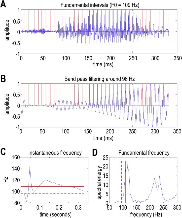
This paper introduces active listening, as a unified framework for synthesising and recognising speech. The notion of active listening inherits from active inference, which considers perception and action under one universal imperative: to maximise the evidence for our (generative) models of the world. First, we describe a generative model of spoken words that simulates (i) how discrete lexical, prosodic, and speaker attributes give rise to continuous acoustic signals; and conversely (ii) how continuous acoustic signals are recognised as words. The 'active' aspect involves (covertly) segmenting spoken sentences and borrows ideas from active vision. It casts speech segmentation as the selection of internal actions, corresponding to the placement of word boundaries. Practically, word boundaries are selected that maximise the evidence for an internal model of how individual words are generated. We establish face validity by simulating speech recognition and showing how the inferred content of a sentence depends on prior beliefs and background noise. Finally, we consider predictive validity by associating neuronal or physiological responses, such as the mismatch negativity and P300, with belief updating under active listening, which is greatest in the absence of accurate prior beliefs about what will be heard next.

Keywords: Audition; Segmentation; Variational Bayes; Voice; active inference; active listening; speech recognition.

Fig. 1

A generative model of a word. This figure illustrates the generative model from the perspective of word generation (green panels) and accompanying inversion (orange panels), which corresponds to word recognition. In brief, the first step—when generating a word—is to construct a time-frequency representation based on the lexical content of the word. This representation is then transformed into distinct transients, which are aggregated to form the acoustic timeseries of the spoken word. For word recognition, the steps are essentially inverted: the timeseries is segregated into transients, which are transformed into a time-frequency representation. The time-frequency representation is used to infer the lexical content of the spoken word. For the equations describing these probabilistic transformations, please see Appendix 1. (For interpretation of the references to colour in this figure legend, the reader is referred to the Web version of this article.)

Fig. 2

Fundamental and formant intervals. This figure illustrates the way in which an acoustic timeseries is generated by assembling a succession of transients separated by an interval that is inversely proportional to the (instantaneous) fundamental frequency. The duration of each transient places an upper bound on the wavelength of the formant frequencies—and corresponds to the minimum frequency, which we take to be the first formant frequency.

Fig. 3

Fundamental frequencies and intervals. This figure illustrates the estimation of fluctuations around the fundamental frequency during the articulation of (the first part of) a word. These fluctuations correspond to changes in the fundamental interval; namely, the reciprocal of the instantaneous frequency. Panel A shows the original timeseries, while Panel B shows the same timeseries after bandpass filtering. The peaks (i.e., phase crossings) then determine the intervals, which are plotted in terms of instantaneous frequencies in Panel C (as a blue line). The solid red line corresponds to the mean frequency (here, 109 Hz), while the broken red line corresponds to the centre frequency of the bandpass filtering (here, 96 Hz) which is centred on the prior for the speaker average fundamental frequency. The same frequencies are shown in panel D (this time on the x-axis), superimposed on the spectral energy (the absolute values of the accompanying Fourier coefficients of the timeseries in Panel A). The ensuing fundamental intervals are visualised as red lines in Panels A and B. (For interpretation of the references to colour in this figure legend, the reader is referred to the Web version of this article.)

Fig. 4

Fundamental and formant frequencies: Both plots show the root mean square power (i.e., absolute value of Fourier coefficients) following the Fourier transform of a short segment of speech. The frequency range in the upper plot covers the first 500 Hz. The first peak in power (illustrated by the blue vertical line) corresponds to the fundamental frequency, which is typically between 80 and 150 Hz for adult men and up to 350 Hz for adult women. The lower panel shows the same spectral decomposition but covers 8000 Hz to illustrate formant frequencies. The solid blue lines show the calculated formant frequency and its multiples, while the grey lines arbitrarily divide the frequency intervals into eight bins. These frequencies define the frequencies used for the spectral decomposition. (For interpretation of the references to colour in this figure legend, the reader is referred to the Web version of this article.)

Fig. 5

Spectral envelopes and segment boundaries. This figure provides an example of how candidate intervals containing words are identified using the spectral envelope. The upper panel shows a timeseries produced by saying "triangle, square". The timeseries is high pass filtered and smoothed using a Gaussian kernel. The red line in the upper panel shows the resulting spectral envelope, after subtracting the minimum. This envelope is reproduced in the lower panel (red line). The horizontal blue line corresponds to a threshold: 1/16th of the maximum encountered during the (1250 ms) epoch. Boundaries are then identified as the first crossing (black dot) of the threshold (horizontal blue line) before the spectral peak and the last crossing after the peak. These boundaries are then supplemented with the internal minima between the peak and offset (red dots). These boundaries then generate a set of intervals for subsequent selection during the recognition or inference process. Here, there are three such intervals. The first contains the first two syllables of triangle, the second contains the word "triangle". The third additionally includes the first phoneme of "square". In this example, the second interval was selected as the most plausible (i.e., free energy reducing) candidate to correctly infer that this segment contained the word "triangle". The vertical blue line corresponds to the first spectral peak following the offset of the last word, which provides a lower bound on the onset. (For interpretation of the references to colour in this figure legend, the reader is referred to the Web version of this article.)

Fig. 6

Speech recognition and segmentation. Left panel: This panel shows the results of active listening to a sequence of words: a succession of “triangle, square, triangle, square …. ”. Its format will be used in subsequent figures and is described in detail here. Panel A shows the acoustic timeseries as a function of time in seconds. The different colours correspond to the segmentation selected by the active listening scheme, with each colour corresponding to an inferred word. Regions of cyan denote parts of the timeseries that were not contained within a word boundary. Panel B shows the accompanying spectral envelope (back line) and the threshold (red dashed line) used to identify subsequent peaks. The first peak of each successive word centres the boundary identification scheme of Panel A. The words that have been inferred are shown in the same colours as the upper panel at their (inferred) onset. Panels C–D show the results of simulated neuronal firing patterns and local field potentials or electroencephalographic responses. These are based upon a simple form of belief updating cast as a neuronally plausible gradient descent on variational free energy (please see main text). Panel C shows the activity of neuronal populations encoding each potential word (here, 14 alternatives listed on the Y axis). These are portrayed as starting at the offset of each word. Effectively, these reflect a competition between lexical representations that record the selection of the most likely explanation. Sometimes this selection is definitive: for example, the first word (“triangle”) supervenes almost immediately. Conversely, some words induce a belief updating that is more uncertain. For example, the last word (“red”) has at least three competing explanations (i.e., “no”, “not” and “a”). Even after convergence to a particular posterior belief, there is still some residual uncertainty about whether “red” was heard. Note that the amplitude of the spectral envelope is only just above threshold. In other words, this word was spoken rather softly. Panel D shows the same data after taking the temporal derivative and filtering between 1 and 16 Hz. This reveals fluctuations in (simulated) depolarisation that drives the increases or decreases in neuronal firing of the panels above. In this example, the sequence of words was falsely inferred to be a mixture of several words not actually spoken. This failure to recognise the words reflects the fact that the sequence was difficult to parse or segment. Once segmentation fails, it is difficult to pick up the correct sequence of segmentations that will, in turn, support veridical inference. These results can be compared with the equivalent results when appropriate priors are supplied to enable a more veridical segmentation and subsequent recognition. Right panel: This panel shows the results of active listening using the same auditory stream as in the left panel. The only difference here is that the (synthetic) subject was equipped with strong prior beliefs that the only words in play were either “triangle” or “square”. This meant that the agent could properly identify the succession of words, by selecting the veridical word boundaries and, by implication, the boundaries of subsequent words. If one compares the ensuing segmentation with corresponding segmentation in the absence of informative priors, one can see clearly where segmentation failed in the previous example. For example, the last word (i.e., “square”) is correctly identified in dark blue in Panel F. Whereas, in Panel B (without prior constraints), the last phoneme of the word “square” was inferred as "red" and the first phoneme was assigned to a different word (“is”). The comparative analysis of these segmentations highlights the ‘handshake’ between inferring the boundaries in a spectral envelope and correctly inferring the lexical content on the basis of fluctuations in formant frequencies. (For interpretation of the references to colour in this figure legend, the reader is referred to the Web version of this article.)

Fig. 7

The role of priors in a word recognition: This figure uses the same format as Fig. 6. In this example, the spoken sentence was “Is there a square above?” The left panel (A–D) shows the results of segmentation and word recognition under informative priors about the possible words. In other words, for each word in the sequence, a small number of plausible options were retained for inference. For example, the word “above” could have been “below” or “there”, as shown by the initial neuronal firing in Panel C at the end of the last word (red arrow). The right panel (E–H) shows exactly the same results but in the absence of any prior beliefs. The inference is unchanged; however, one can see in the neuronal firing (Panel G) that other candidates are competing to explain the acoustic signal (e.g., blue arrows). The key observation is that the resulting uncertainty—and competition among neuronal representations—is expressed in terms of an increased amplitude of simulated electrophysiological responses. This can be seen by comparing the simulated EEG trace in Panel H—in the absence of priors (solid lines)—with the equivalent EEG response under strong priors (solid lines in Panel D, reproduced as dashed lines in Panel H). In this example, there has been about a 50% increase in the amplitude of evoked responses. A more detailed analysis of the differences in simulated EEG responses is provided in Fig. 8. (For interpretation of the references to colour in this figure legend, the reader is referred to the Web version of this article.)

Fig. 8

Mismatch responses and speech-in-noise: Panel A reproduces the results of Fig. 7H, but focuses on the simulated electrophysiological responses of a single neuronal population responding to the third word (“a”). The upper row reports simulated responses evoked with (green lines) and without (blue dashed lines) priors (as in Fig. 7), while the lower row shows the differences between these two responses. These differences can be construed in the spirit of a mismatch negativity or P300 waveform difference. Removing the priors over the third word (Panels C–D) isolates the evoked responses and their differences more clearly. The grey shaded area corresponds to a peristimulus time of 500 ms, starting 250 ms before the offset of the word in question. Assuming update time bins of around 16 ms means that we can associate this differential response with a P300. In other words, when the word is more surprising—in relation to prior beliefs about what will be heard—they evoke a more exuberant response some 300 ms after its offset. Panels E–H report the same analysis with one simple manipulation; namely, the introduction of noise to simulate speech-in-noise. In this example, we doubled the amount of noise; thereby shrinking the coefficients by about a factor of half. This attenuates the violation (i.e., surprise) response by roughly a factor of two (compare difference waveform in Panel D without noise—red arrows—with the difference waveform in Panel H without noise—blue arrow). Interestingly, in this example, speech-in-noise accentuates the differences evoked in this simulated population when the word is not selected (i.e., on the previous word). The underlying role of surprise and prior beliefs in determining the amplitude of these responses is addressed in greater detail in the final figure. (For interpretation of the references to colour in this figure legend, the reader is referred to the Web version of this article.)

Fig. 9

Recursive recognition and generation: The upper part of this figure shows the recognition of words (Panel B) contained within an acoustic signal (Panel A). Here, the acoustic signal is parsed into the words “is there a square above”. The corresponding lexical states can be used to synthesise a new acoustic signal (Panel C) containing the same words. Here, we inverted the model a second time, to recover the words contained within the synthetic acoustic signal (Panel D). Happily, the recovered words from the synthetic signal (Panel D) match those from the original signal (Panel B).

Fig. 10

Bayesian surprise and evoked responses: this shows the same results as in Fig. 7 but after removing priors from the third word (“a” in blue). Panel A shows the acoustic timeseries and Panels B–C show the results of simulated neuronal firing patterns and simulated electroencephalographic responses. The result is a more vigorous (simulated) event related response after the onset of the third word (green line in Panel C). A simple measure of these surprise-related responses can be obtained by taking the variance of the (simulated) responses over all populations as a function of time (c.f., evoked power). This is shown in Panel D as a solid blue line (normalised to a maximum of four arbitrary units). The red bars in Panel D correspond to the degree of belief updating or Bayesian surprise, as measured by the KL divergence between prior and posterior beliefs after updating. The key conclusion from these numerical analyses is that there is a monotonic relationship between the evoked power and Bayesian surprise, reflected by the nearly linear relationship between Bayesian surprise and the maxima of evoked power in Panel E. In short, the greater the Bayesian surprise, the greater the belief updating and the larger the fluctuations in neuronal activity. (For interpretation of the references to colour in this figure legend, the reader is referred to the Web version of this article.)

Fig. 11

A generative model of a word. This figure illustrates the generative model from the perspective of word generation (green panels) and accompanying inversion (orange panels), which corresponds to word recognition. This model maps from hidden states (s; shown in box A), which denote the attributes of a spoken word (in this case lexical content, prosody, and speaker identity), to outcomes (o; shown in box C), which corresponds to the continuous acoustic timeseries. Box B shows how parameters are sampled for word generation. The centre panels illustrate the non-linear mappings between model parameters and the acoustic spectrum (i.e., time-frequency representation). Box C specifies how the transients are then aggregated to form a timeseries. Recognition (boxes D–E) corresponds to the inversion of the generative model: a given time series is transformed to parameterise the time-frequency representation (box D) by simply inverting or ‘undoing’ the generative operations. These parameters are used to evaluate the likelihood of lexical, prosody and speaker states (box E). The equations displayed in this figure are unpacked in the text.

Fig. 12

A graphical formulation of the generative model. This figure illustrates the same model as described in Fig. 11, but uses a normal (Forney) factor graph form. This graphical notation relies upon the factorisation of the probability density that underwrites the generative model. Each factor is specified in the panel on the left. Factor 1 is the prior probability associated with the hidden states and takes a categorical form. Factor 2 is a normal distribution that specifies the dependence of parameters on states. Each discrete state is associated with a different expectation and covariance for the parameters. Factor 3 describes how the observed timeseries is generated from the parameters, and this is decomposed into factors 4–9. These are Dirac delta functions that may be thought of as normal distributions, centred on zero, with infinite precision (i.e., zero covariance). In the graphs on the right, factors are indicated by numbered squares, and these are connected by edges (Hasson et al., 2008), which represent the variables common to the factors they connect. The upper right graph shows factors 1–3, and the lower graph unpacks factor 3 in terms of factors 4–9. The process of generating data may be thought of in terms of a series of local operations taking place at each factor from top to bottom (i.e., sample states from factor 1, then parameters from factor 2, then perform the series of operations in factor 3 to get the timeseries). The recognition process can be thought of as bidirectional message passing across each factor node, such that empirical priors and likelihoods are combined at each edge to form posterior beliefs about the associated variable. Factor 5 is of particular interest here, as it determines the internal ‘action’ that selects the interval for segmentation.

References

1. Abberton E., Fourcin A.J. Intonation and speaker identification. Lang. Speech. 1978;21(4):305–318. - PubMed
1. Adams R.A., Shipp S., Friston K.J. Predictions not commands: active inference in the motor system. Brain Struct. Funct. 2013;218(3):611–643. - PMC - PubMed
1. Aitchison L., Lengyel M. With or without you: predictive coding and Bayesian inference in the brain. Curr. Opin. Neurobiol. 2017;46:219–227. - PMC - PubMed
1. Alain C., Arnott S.R., Hevenor S., Graham S., Grady C.L. “What” and “where” in the human auditory system. Proc. Natl. Acad. Sci. Unit. States Am. 2001;98(21):12301–12306. - PMC - PubMed
1. Altenberg E.P. The perception of word boundaries in a second language. Sec. Lang. Res. 2005;21(4):325–358.
Publication types