High-acuity vision from retinal image motion

Abstract

A mathematical model and a possible neural mechanism are proposed to account for how fixational drift motion in the retina confers a benefit for the discrimination of high-acuity targets. We show that by simultaneously estimating object shape and eye motion, neurons in visual cortex can compute a higher quality representation of an object by averaging out non-uniformities in the retinal sampling lattice. The model proposes that this is accomplished by two separate populations of cortical neurons - one providing a representation of object shape and another representing eye position or motion - which are coupled through specific multiplicative connections. Combined with recent experimental findings, our model suggests that the visual system may utilize principles not unlike those used in computational imaging for achieving "super-resolution" via camera motion.

Figure 1.

Model Overview: (A) An upright letter E (stroke width = 0.8 arcmin) projected onto a simulated cone lattice (average spacing 1.09 arcmin) with a 500 ms eye drift trajectory (Ratnam et al., 2017) superimposed (green trace). RGC cell spikes are generated using a linear-nonlinear-poisson model with ON and OFF cells. The ON and OFF RGC response functions are symmetrical, so the presence of a stimulus for an ON cell gives an equivalent response to the absence of a stimulus for an OFF cell. (B) Probabilistic model for inferring stimulus shape S (encoded by latent variables A) and position X from retinal spikes R. Arrows indicate causal relationships between variables. The spikes R are observed and the latent factors encoding shape A and position X must be simultaneously inferred. (C, D) The spike decoder repeatedly alternates between two steps: (C) In the first step (Equations 5), the estimate of the pattern is fixed (S = S^t) and new evidence coming from the next set of incoming spikes R_{t + 1} is incorporated to obtain an updated posterior distribution over eye position P(X_{t + 1}|R_{0: t + 1}) (shown as a probability cloud). This update is computed by multiplying the probability distribution over the predicted position P(X_{t + 1}|R_{0: t}) (computed from the diffusion model applied to the previous position estimate) together with the likelihood P(R_{t + 1}|X_{t + 1}, S = S^t) (computed by cross-correlating the current estimate of the pattern with the spatial array of incoming spikes). (D) In the second step (Equations 8, 10), the neurons representing the internal position estimate X_t act to dynamically route incoming spikes by multiplicatively gating their connections to the internal pattern estimate, thus updating S.

Figure 2.

Benefits of motion for the discrimination of high-acuity targets: (A) Stimulus (S) to be recovered. The entire pattern is defined on a 20 × 20 pixel array subtending 8 arcmin. The width of each leg of the E is 2 pixels (0.8 arcmin). The cone lattice and eye trajectories are the same as in Figure 1A. (B) SNR of the reconstruction of the E as a function of time. The Shaded region shows 95% confidence intervals of the mean given 40 trials. Either the stimulus is moved relative to the retina (S:M = Motion), or not (S:NM = No Motion). For each of these cases, the stimulus pattern is inferred using either the approximate EM algorithm (D:EM) or an optimal decoder assuming no motion (D:NM) are used to decode the pattern. Note that D:EM > D:NM, even when there is no stimulus motion (S:NM) because the uncertainty over the position implicitly smooths the pattern. The difference between the two best methods is statistically significant (S:M | D:EM > S:NM | D:EM with p = 0.002 at t = 700 ms). (C) Typical reconstructions of the pattern in the case of either motion and no motion after 700 ms. (D) Reconstruction over time in the case of motion using the EM algorithm. (E) Reconstruction over time in the case of motion assuming no motion. (F) Estimated versus true eye position as a function of time. The red curve shows the estimated horizontal and vertical eye position using the EM algorithm (width reflects +/−1 standard deviation). The blue curve shows the true eye position. The timestep of the simulation is 1 ms.

Figure 3.

Motion benefit during cone loss. (A) Letter E stimulus sampled by a retinal cone lattice that has 30% of the cones dropped out randomly (cone loss, eye trajectories, and RGC spikes are resampled each trial). The same stimulus size, cone spacing, eye trajectories, and diffusion constant for inference were used as in Figure 2. (B) SNR at t = 700 ms as a function of cone loss for a moving and a stationary retina with n = 21 for each motion condition and cone loss value. The error bars correspond with plus or minus one standard error of the mean. (C and D) Examples of the reconstructed stimulus in the case of retinal drift motion and no motion for 30% cone loss.

Figure 4.

Neurons with structured receptive fields improve inference. (A) A whitened 32 × 32 pixel natural scene patch scaled to subtend a square with side length 24 arcmin is projected onto a simulated cone lattice with an average spacing of 1 arcmin. The retinal drift motion in this case is generated by a random walk with $D_c=20{\text{arcmin}}^2/s$. (B) SNR of the decoded image at t = 600 ms. RGC spikes are decoded using three pattern priors. The SNR is plotted relative to PCA averaged over 15 trials (different natural scene patches and eye trajectories). Error bars show 95% confidence intervals. The p-values are calculated between the uniform prior and PCA, and between the sparse coding prior and PCA (**** p < 0.0001; *** p < 0.001). (C) A random set of 25 elements from the learned sparse coding dictionary, D. Sparse coding seeks to describe any given image pattern as a sparse linear combination of these features. (D – F) Example reconstructed image patterns for each method after 600 ms. IND, independent pixel prior; PCA, Gaussian prior; SP, dictionary trained with sparse coding with both a L1 and L2 prior.

Figure 5.

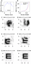
Extended Tuning Plots: (A) The SNR as a function of motion gain (n = 40 for each value of the motion gain). The experimentally measured eye trajectories are used, except that the overall position is multiplied by the gain factor. (B) The SNR as a function of stimulus size (n = 20). Both plots use the same parameters as in Figure  2. The error bars in both plots show the standard error. (E–H) Example reconstructions for the stimulus size experiments with stroke width (w), and motion (S:M) or no motion (S:NM). The horizontal and vertical axes are in arcmin. (C, D) For small stimuli, the orientation of the stimulus is unrecognizable in both cases. (E, F) For stimuli with a stroke width on the order of the spacing of the cones, the orientation of the stimulus is barely recognizable. (G, H) For larger stimuli, although the SNRs are different, the orientation of the stimulus is unambiguous, despite a large difference in the SNR.

References

1. Ahmad K. M., Klug K., Herr S., Sterling P., & Schein S. (2003). Cell density ratios in a foveal patch in macaque retina. Visual Neuroscience, 20(02), 189–209. - PubMed
1. Anderson C. H., & Van Essen D. C. (1987). Shifter circuits: a computational strategy for dynamic aspects of visual processing. Proceedings of the National Academy of Sciences of the United States of America, 84(17), 6297–6301. - PMC - PubMed
1. Arathorn D. W., Stevenson S. B., Yang Q., Tiruveedhula P., & Roorda A. (2013). How the unstable eye sees a stable and moving world. Journal of Vision, 13(10), 22. - PMC - PubMed
1. Aytekin M., Victor J. D., & Rucci M. (2014). The visual input to the retina during natural head-free fixation. Journal of Neuroscience, 34(38), 12701–12715. - PMC - PubMed
1. Beck A., & Teboulle M. (2009). A fast iterative shrinkage-thresholding algorithm for linear inverse problems. SIAM Journal on Imaging Sciences, 2(1), 183–202.
Publication types