Listeria monocytogenes contamination of ready-to-eat foods and the risk for human health in the EU

Abstract

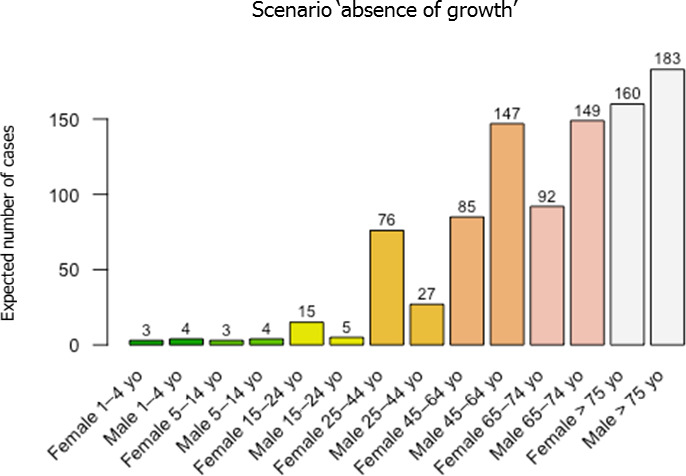
Food safety criteria for Listeria monocytogenes in ready-to-eat (RTE) foods have been applied from 2006 onwards (Commission Regulation (EC) 2073/2005). Still, human invasive listeriosis was reported to increase over the period 2009-2013 in the European Union and European Economic Area (EU/EEA). Time series analysis for the 2008-2015 period in the EU/EEA indicated an increasing trend of the monthly notified incidence rate of confirmed human invasive listeriosis of the over 75 age groups and female age group between 25 and 44 years old (probably related to pregnancies). A conceptual model was used to identify factors in the food chain as potential drivers for L. monocytogenes contamination of RTE foods and listeriosis. Factors were related to the host (i. population size of the elderly and/or susceptible people; ii. underlying condition rate), the food (iii. L. monocytogenes prevalence in RTE food at retail; iv. L. monocytogenes concentration in RTE food at retail; v. storage conditions after retail; vi. consumption), the national surveillance systems (vii. improved surveillance), and/or the bacterium (viii. virulence). Factors considered likely to be responsible for the increasing trend in cases are the increased population size of the elderly and susceptible population except for the 25-44 female age group. For the increased incidence rates and cases, the likely factor is the increased proportion of susceptible persons in the age groups over 45 years old for both genders. Quantitative modelling suggests that more than 90% of invasive listeriosis is caused by ingestion of RTE food containing > 2,000 colony forming units (CFU)/g, and that one-third of cases are due to growth in the consumer phase. Awareness should be increased among stakeholders, especially in relation to susceptible risk groups. Innovative methodologies including whole genome sequencing (WGS) for strain identification and monitoring of trends are recommended.

Keywords: Listeria monocytogenes; human listeriosis; quantitative microbiological risk assessment; ready‐to‐eat food products; time series analysis.

Figure 1

Schematic overview of transmission routes and the control system of Listeria monocytogenes in ready‐to‐eat (RTE) foods

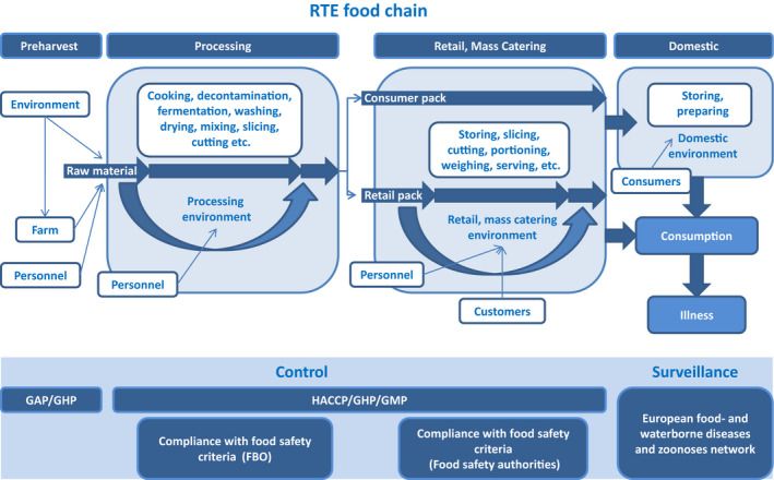
1. FBO: food business operator; GAP: good agricultural practice; GHP: good hygiene practices; GMP: good manufacturing practices; HACCP: hazard analysis and critical control points; RTE: ready‐to‐eat.

2. Consumer pack: food packs that are not processed during retail; retail pack: food packs that are further processed (i.e. sliced) during retail.

Figure 2

Flow chart of the approach to answer the terms of reference

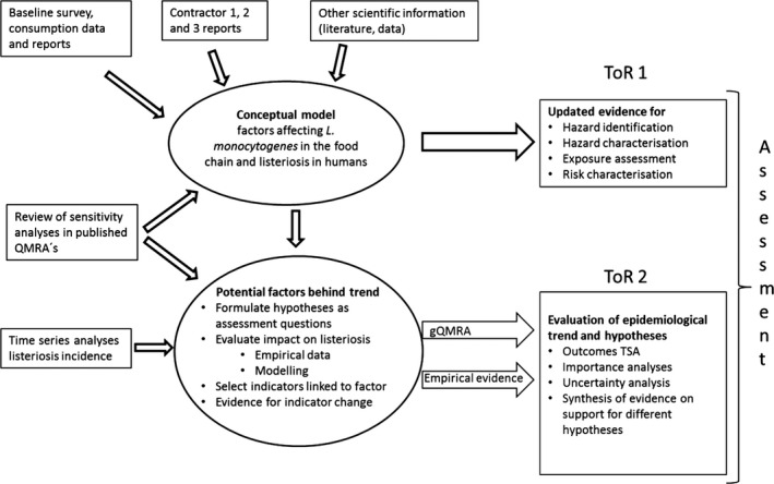
1. gQMRA: generic quantitative microbiological risk assessment; ToR: terms of reference; TSA: time series analyses.

Figure 3

Listeria monocytogenes generic quantitative microbiological risk assessment (gQMRA) model

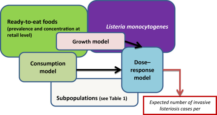
1. The gQMRA model is constructed around three main elements; food, population and hazard. It includes three models: consumption model, growth model and dose–response model. The overlapping of the model boxes with the main element boxes indicates that the model takes into account one or several factors characterising the food, the populations or the hazard.

Figure 4

Empirical cumulative distribution function of L. monocytogenes concentrations per RTE food category based on baseline survey data (EFSA, 2013, 2014a)

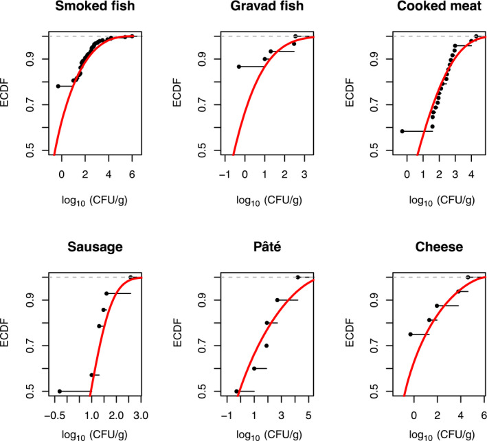
1. For better visibility, different scales of the x‐axis were used. The empirical cumulative distribution function (ECDF) is a step function that jumps up by 1/n at each of the n data points. Its value at any specified value of the measured variable is the fraction of observations of the measured variable that are less than or equal to the specified value. Example: for pâté, curves show that concentration has a probability of 90% to be less or equal to 3 log₁₀ CFU/g. The cumulative distribution function (solid red line) is the probability that the concentration will take a value less than or equal to a specific concentration. Example: for smoked fish, the concentration has a probability of around 90% to be less or equal to 2 log₁₀ CFU/g.

Figure 5

Fitted cumulative distribution functions of L. monocytogenes concentrations per RTE food subcategory obtained from the US data (Gombas et al. (2003)) and the baseline survey data

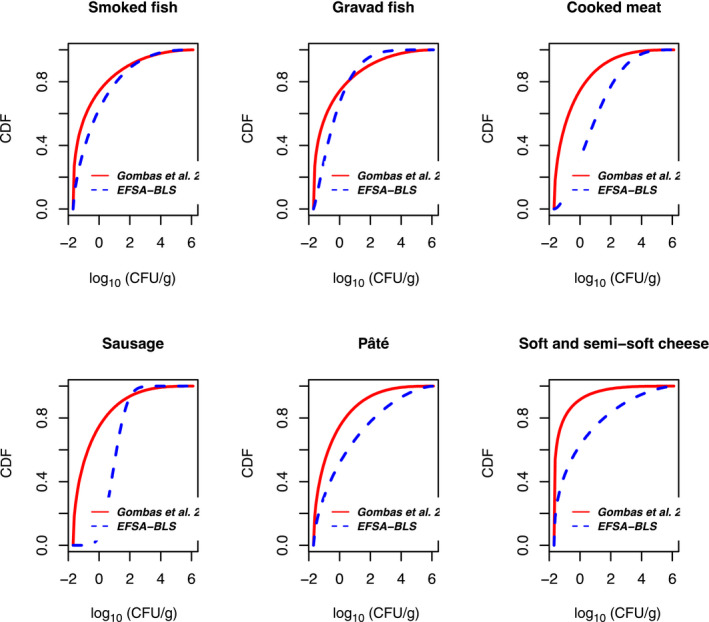
1. The cumulative distribution function is the probability that the concentration will take a value less than or equal to a specific concentration. Example: the blue dashed curve shows that for smoked fish, the concentration has a probability of around 90% to be less or equal to 2 log₁₀ CFU/g.

Figure 6

Example of simulated doses distribution (log₁₀ CFU of L. monocytogenes per eating occasions) in a generic ready‐to‐eat (RTE) food based on using option 3 for the initial concentration of L. monocytogenes in the seven RTE food subcategories considered

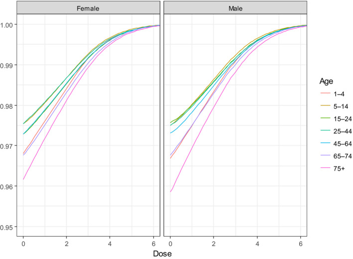
1. The y‐axis represents the cumulative distribution function. This is the probability that the concentration will take a value less than or equal to a specific concentration. Example: the curve in the male population ‘above 75 years old’ shows that the concentration in the generic RTE food has a probability of around 98% to be less than or equal to 2 log₁₀ CFU/g. Option 3: using fish products distribution from EU BLS data, and meat and cheese distributions from US data (Gombas et al., 2003).

Figure 7

Number of confirmed human invasive listeriosis cases/100,000 population by age group and gender in the EU/EEA in 2015

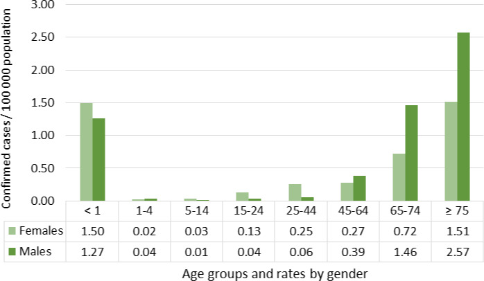
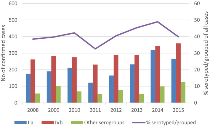
1. Source: Data from The European Surveillance System – TESSy, provided by Austria, Belgium, Croatia, Cyprus, the Czech Republic, Denmark, Estonia, Finland, France, Germany, Greece, Hungary, Iceland, Ireland, Latvia, Lithuania, Luxembourg, Malta, the Netherlands, Norway, Poland, Portugal, Romania, Slovakia, Slovenia, Spain, Sweden, the United Kingdom and released by ECDC.

Figure 8

Distribution of clonal complexes (CCs) as assigned by whole genome sequencing in ready‐to‐eat foods and from sporadic human clinical infections (a) and from the three major food product categories (b) from Møller et al. (2017)

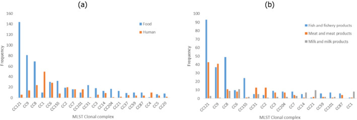
1. The y‐axis represents the number of isolates.

Figure 9

Case fatality rates in different age–gender groups in invasive human infections with Listeria monocytogenes serogroup IIa (a) and serogroup IVb (b), pooled data, 2007–2015

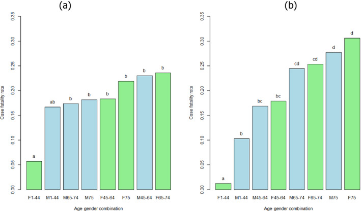
1. F: female (green bar); M: male (blue bar).

2. Case fatality rate values not significantly different have the same letter (comparisons only within groups). Multiple comparison analysis conducted in each serogroup separately with alpha = 0.1.

Figure 10

Dose–response models (probability of severe listeriosis cases conditional to the exposed dose) for each of the 11 population segments considered in Pouillot et al. (2015b)

Figure 11

Proportion of single samples at processing (a) and retail (b) non‐compliant with EU Listeria monocytogenes food safety criteria based on the monitoring data collected by EFSA, 2008–2015

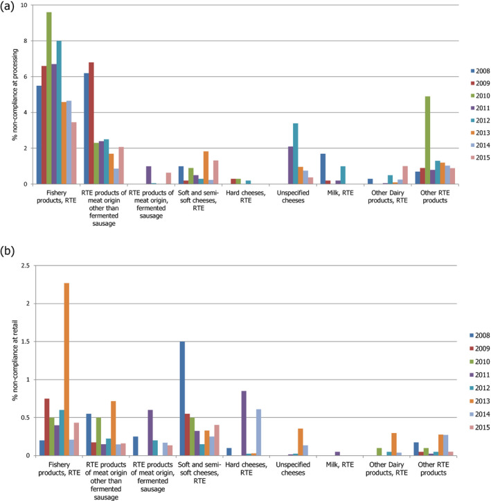
1. RTE: ready‐to‐eat. This graph includes data where sampling stage at retail (also catering, hospitals and care homes) and at processing (also cutting plants) have been specified for the relevant food types. Data collected at the ‘unspecified’ sampling stage are included in the data reported at retail. The category ‘other RTE products’ includes RTE food other than: ‘RTE fishery products,’ ‘soft and semi‐soft cheese,’ ‘hard cheese,’ ‘unspecified cheese,’ ‘other RTE dairy products,’ ‘milk,’ ‘RTE products of meat origin other than fermented sausage,’ ‘RTE products of meat origin, fermented sausage.’ For the non‐compliance analysis of samples collected at the processing stage, the food safety criterion of ‘absence in 25 g’ was applied, except for samples of hard cheese and fermented sausage that were assumed to be unable to support the growth of L. monocytogenes and for which the criterion of ‘≤ 100 CFU/g’ was applied. For the non‐compliance analysis of samples collected at the retail level, the FSC of ‘≤ 100 CFU/g’ was applied. Only information on the main RTE food categories (RTE fishery products, RTE cheese and RTE meat products) is included in this graph. The number of samples at processing ranged from year to year from 456 to 13,578 for ‘RTE fishery products’, from 1,132 to 40,853 for ‘RTE products of meat origin other than fermented sausage’, from 14 to 1,283 for ‘RTE products of meat origin, fermented sausage’, from 585 to 8,381 for ‘soft and semi‐soft cheese’, from 220 to 5,897 for ‘hard cheese’, from 1,365 to 4,264 for ‘unspecified cheese’, from 111 to 1,890 for ‘milk, RTE’, from 312 to 5,418 for ‘other RTE dairy products’, and from 57 to 2,397 for ‘other RTE products’. The number of samples at retail ranged from year to year from 1,356 to 7,174 for ‘RTE fishery products’, from 3,264 to 16,653 for ‘RTE products of meat origin other than fermented sausage’, from 85 to 2,772 for ‘RTE products of meat origin, fermented sausage’, from 699 to 4,381 for ‘soft and semi‐soft cheese’, from 245 to 2,058 for ‘hard cheese’, from 283 to 4,598 for ‘unspecified cheese’, from 48 to 2,766 for ‘milk, RTE’, from 605 to 5,110 for ‘other RTE dairy products’, and from 9,786 to 16,208 for ‘other RTE products’.

Figure 12

Box‐plot showing the Listeria monocytogenes prevalence of ready‐to‐eat (RTE) foods by subcategory

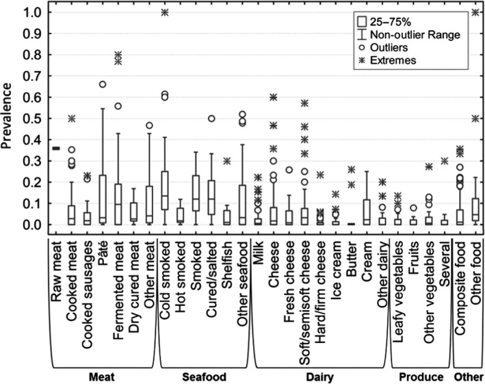
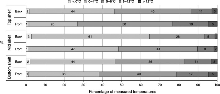
1. Median value is indicated by the line within the interquartile box. Outliers (O) and extreme (⋄) values correspond to values at 1.5‐ and 3‐fold the interquartile range, respectively, from the 75th percentile.

Figure 13

Empirical cumulative distribution function of the reported Listeria monocytogenes concentration in RASFF notifications (2008–2016) for ‘fish and fish products’ (N = 130), ‘milk and milk products’ (N = 126) and ‘meat and meat products other than poultry’ (N = 81)

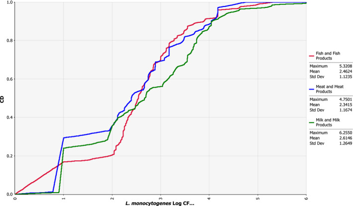
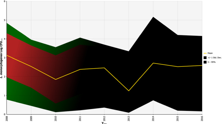
1. The empirical cumulative distribution function is a step function that jumps up by 1/n at each of the n data points. Its value at any specified value of the measured variable is the fraction of observations of the measured variable that are less than or equal to the specified value. Example: the red curve shows that concentration has a probability of 20% to be less or equal to 2 log₁₀ CFU/g.

Figure 14

Temperature distribution (per cent) at the back and front of three different shelves (top, middle and bottom) in 1,812 refrigerators (adopted from Marklinder and Eriksson (2015) © Emerald Group Publishing Limited all rights reserved)

Figure 15

Monthly human cases of confirmed invasive human listeriosis in function of time observed in the EU/EEA, 2008–2015

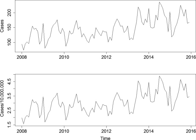
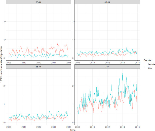
1. Top graph: human invasive listeriosis cases; bottom graph: human invasive listeriosis cases per 10,000,000 population.

Figure 16

Monthly cases of confirmed human invasive listeriosis in function of time observed in the EU/EEA with several additional measures from the fitted model, 2008–2015

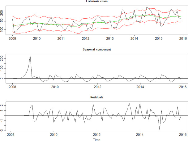
1. Top graph: cases with fitted random walk plus seasonal model and 95% credibility interval (red), and smoothed estimate (green). Middle graph: Seasonal component of the Listeria time series. Bottom graph: Standardised residuals of the Listeria time series after removal of the seasonal component and the trend.

Figure 17

Cases of confirmed human invasive listeriosis in function of time observed in the EU/EEA and future predictions based on the fitted random walk plus seasonal model, with the respective intervals based on one standard deviation, 2008–2015

Figure 18

Evolution of reported human invasive listeriosis incidence rates in the EU/EEA by age and gender, 2008–2015

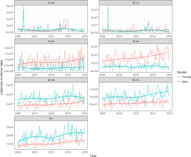
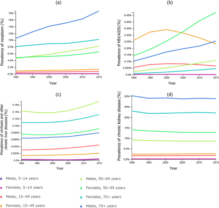
1. The thick lines correspond to smoothed trend lines based on local regression.

Figure 19

A conceptual model describing important factors and processes related to different stages in the food chain (green boxes), consumers (orange box), the epidemiological system (red box), and trade patterns (yellow box) and how they combine (grey boxes and arrows) to influence Listeria monocytogenes contamination, ingested dose, dose–response relationships and the incidence rates of reported human listeriosis

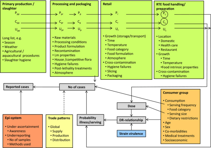
1. C: concentration; Lm: Listeria monocytogenes; P: prevalence; U: food unit size, which may affect the distribution of Lm, i.e. P, and C, considerably. The subscript for C, P and U refers to the production stage.

Figure 20

Expected number of human invasive listeriosis cases per subpopulation and per year in the EU/EEA (1 million iterations) with a scenario ‘absence of growth’

Figure 21

Cumulative risk attribution of human invasive listeriosis per subpopulation for the considered ready‐to‐eat food subcategories

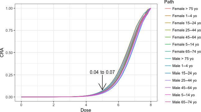
1. The cumulative attribution risk for a specific dose (x) is the proportion of human invasive listeriosis cases attributable to doses lower or equal to x.

Figure 22

Increase in risk of human invasive listeriosis as a function of (a) the mode of the proportion of the remaining shelf life used to store ready‐to‐eat (RTE) food in the consumer refrigerator (using simulations with a maximum proportion equal to 1.1); (b) the maximum of the proportion of remaining shelf life time used to store RTE food in the consumer refrigerator (using simulations with a mode of the proportion equal to 0.3); (c) the mean of the mean temperature of the consumer refrigerator; (d) the maximum population density shift

Figure 23

Prevalence data for L. monocytogenes in the three major RTE food categories based on literature data for the period 1989–2013

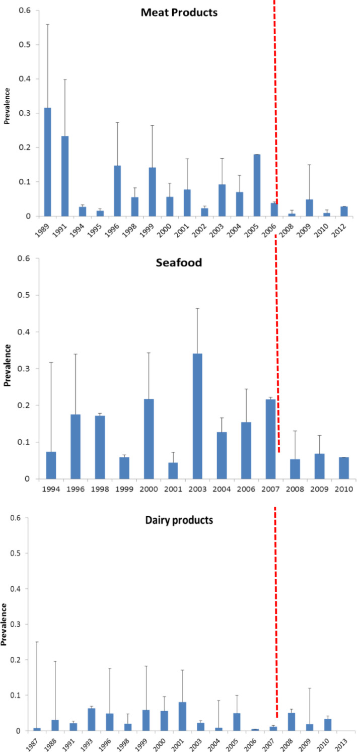
1. Red vertical line shows the beginning of the targeted period of concern for the present Scientific Opinion extending from 2008 onwards. This period is also characterised by scarcity of data.

Figure 24

Summary trend graph for Listeria monocytogenes concentration in ‘fish and fish products’ reported in RASFF notifications for the years 2008–2016

Figure 25

Summary trend graph for Listeria monocytogenes concentration in ‘meat and meat products other than poultry’ reported in RASFF notifications for the years 2008–2016

Figure 26

Summary trend graph for Listeria monocytogenes concentration in ‘milk and milk products’ reported in RASFF notifications for the years 2008–2016

Figure 27

Number of reported Listeria monocytogenes serogroup IIa cases (N = 1,679), serogroup IVb cases (N = 2,329) and cases with other serogroups (N = 632); and proportion of all cases reported with serotype/group data per year in four EU countries, 2008–2015

1. Source: Data from The European Surveillance System – TESSy, provided by Austria, France, Germany, the United Kingdom, and released by ECDC (N = 4,640).

Figure 28

Prevalence (in percentage) in specific age–gender groups in western Europe, 1990–2015, of neoplasm (a), human immunodeficiency virus infection and acquired immune deficiency syndrome (HIV/AIDS) (b), cirrhosis and other chronic liver diseases (c), and chronic kidney disease (d) Data from http://www.healthdata.org/

Figure 29

Annual invasive listeriosis incidence rate (cases/million) (a), annual number of human invasive listeriosis cases (b) and population change (c) per category of age for females

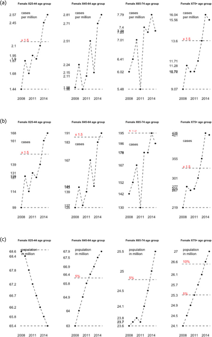
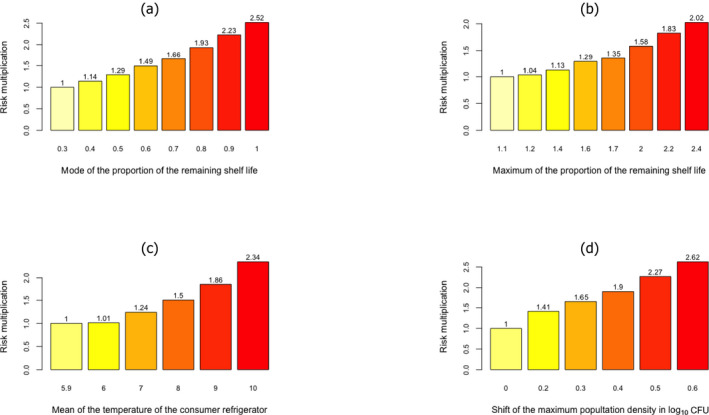
1. The line 1.5 shows the increase from the lowest level by a factor of 1.5, lines 5% and 10% by a percentage of 5 and 10% respectively.

Figure 30

Annual invasive listeriosis incidence rate (cases/million) (a), annual number of human invasive listeriosis cases (b) and population change (c) per category of age for males

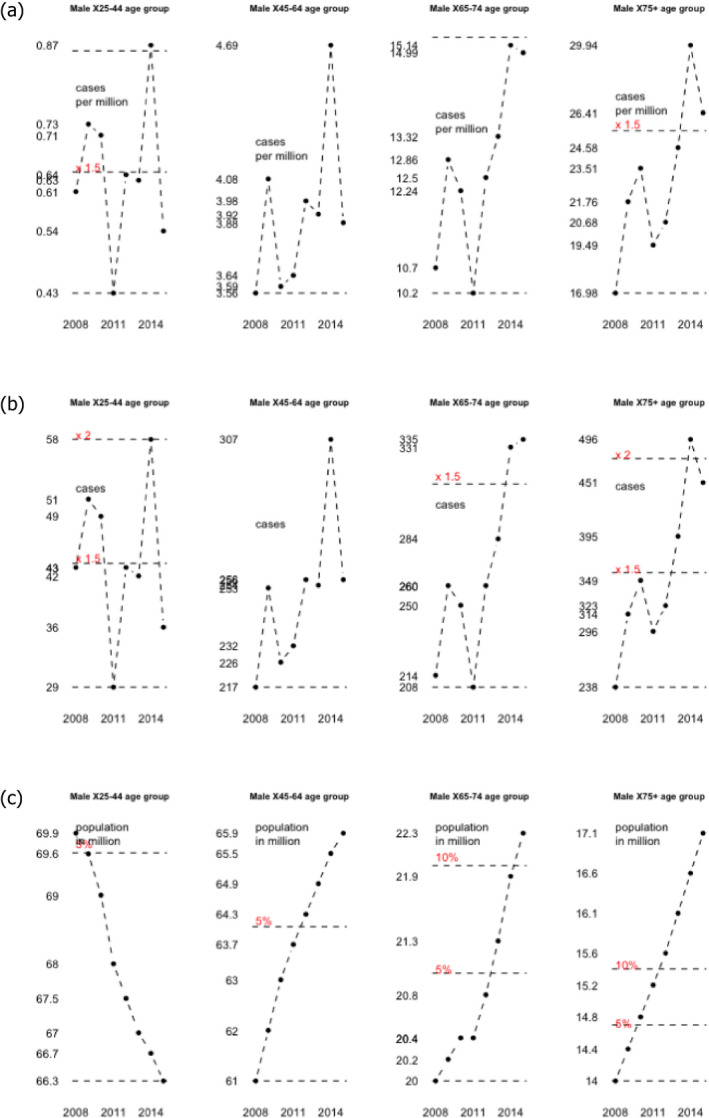
1. The lines 1.5 and 2 show the increase from the lowest level by a factor of 1.5, lines 5% and 10% by a percentage of 5 and 10% respectively.

Figure 31

Expected number of human invasive listeriosis cases per subpopulation and per year using three options for the initial concentration of L. monocytogenes in the seven RTE food subcategories (1 million iterations)

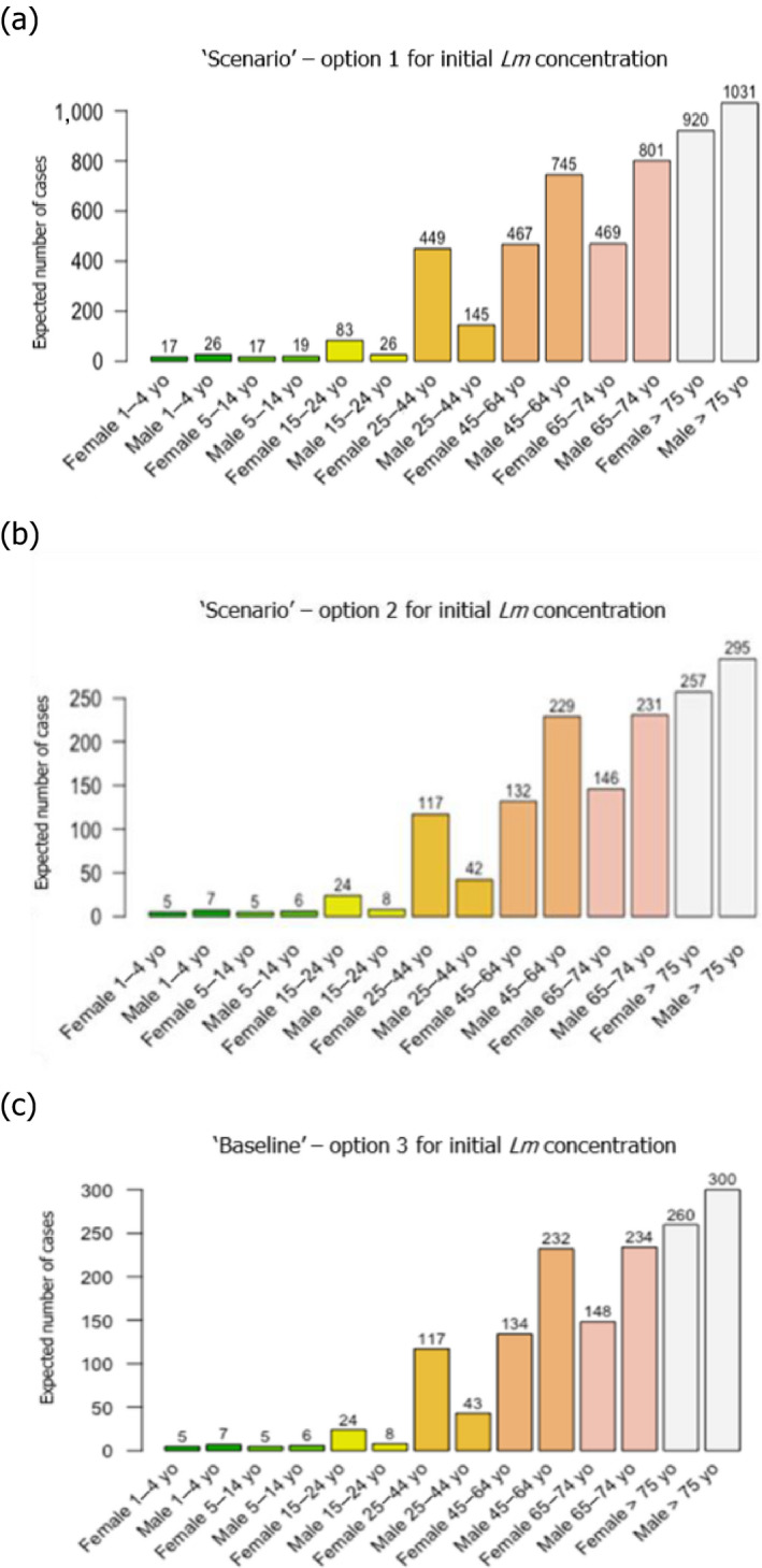
1. (a) Option 1: using only the distributions estimated with BLS data; (b) option 2: using only the distributions estimated with US data (Gombas et al., 2003); and (c) option 3: using fish distribution from BLS data, and meat and cheese distributions from US data (Gombas et al., 2003).

Figure B.1

Evolution of reported human invasive listeriosis incidence rates (cases per month/1,000,000 population) in the EU/EEA, by gender for a selection of age groups, 2008–2015

Figure C.1

Example of simulated doses distribution (log₁₀ CFU of L. monocytogenes per eating occasions) using three options for the initial concentration of L. monocytogenes in three RTE food subcategories

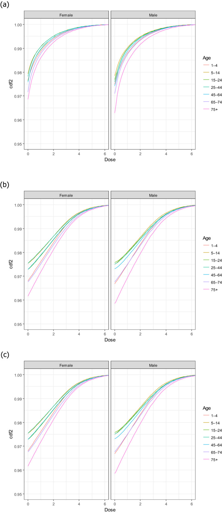
1. CDF: cumulative distribution function. (a) Option 1: using only the distributions estimated with BLS data; (b) Option 2: using only the distributions estimated with US data (Gombas et al., 2003); and (c) Option 3: using fish distribution from EU BLS data, and meat and cheese distributions from US data (Gombas et al., 2003).

Figure H.1

Reported growth/no‐growth interfaces of Listeria monocytogenes at 4°C (upper) and 10°C (lower) with respect to pH and a_w, as predicted at a probability level of 0.1 by four different available models developed using different strains

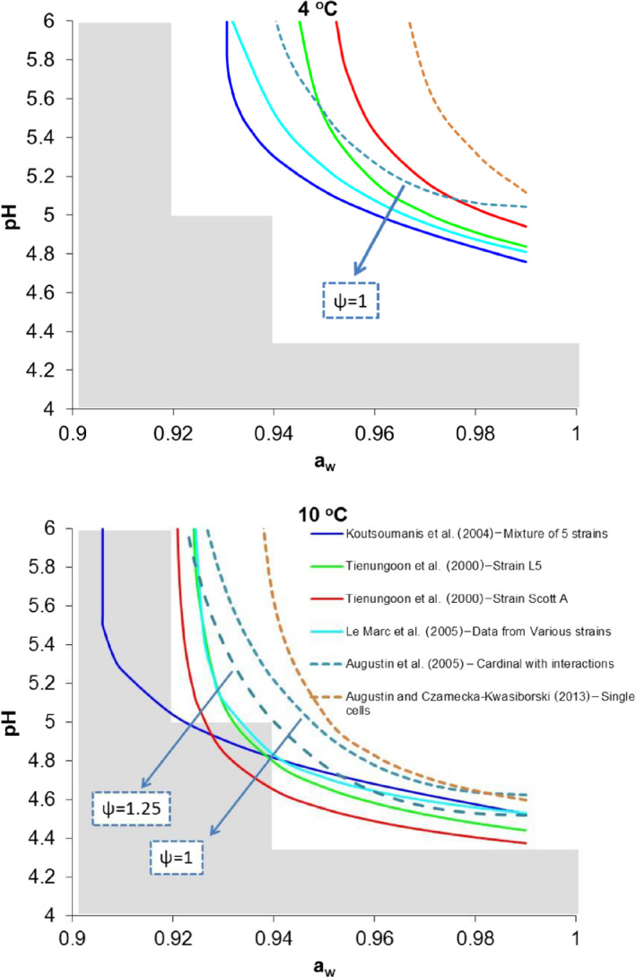
1. Note: Psi‐values greater than 1 indicate the predicted no‐growth zone based on a cardinal model with interactions (Augustin et al., 2005). Shaded area indicate pH and a_w combination defined in Regulation (EC) No 2073/2005 as conditions that do not allow growth of L. monocytogenes (pH ≤ 4.4 or a_w ≤ 0.92, or pH ≤ 5.0 and a_w ≤ 0.94).

References

-
- ACMSF (Advisory Committee on the Microbiological Safety of Food), 2009a. Ad hoc group on vulnerable groups. Report on the increased incidence of listeriosis in the UK. Food Standards Agency, 92 pp. FSA/1439/0709. Available online: https://www.food.gov.uk/sites/default/files/multimedia/pdfs/committee/ac...
- ACMSF (Advisory Committee on the Microbiological Safety of Food), 2009b. Discussion paper report of the Social Science Research Committee Working Group on Listeria monocytogenes and the food storage and food handling practices of the over 60s at home. Food Standards Agency, Social Science Research Committee, 42 pp. ACM/954. Available online: https://www.food.gov.uk/sites/default/files/multimedia/pdfs/committee/ac...,
- Afchain AL, Derens E, Guilpart J and Cornu M, 2005. Statistical modelling of cold‐smoked salmon temperature profiles for risk assessment of Listeria monocytogenes. Proceedings of the 3rd International Symposium on Applications of Modelling as an Innovative Technology in the Agri‐Food Chain. 10.17660/actahortic.2005.674.47, pp. 383–388. - DOI
LinkOut - more resources
Full Text Sources