Low-dose spectral CT reconstruction using image gradient ℓ 0-norm and tensor dictionary

Abstract

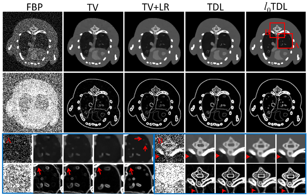
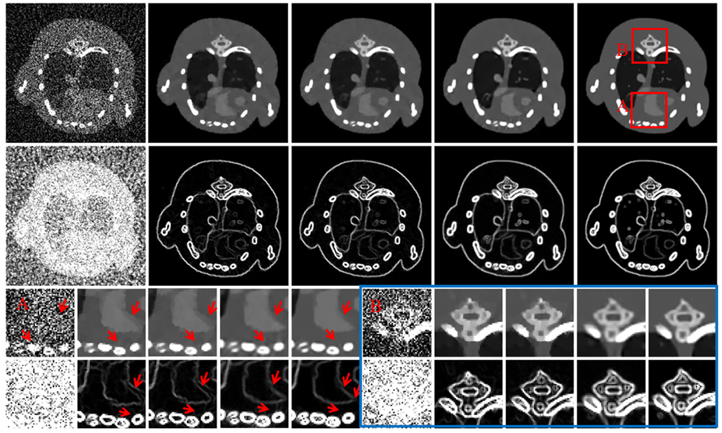
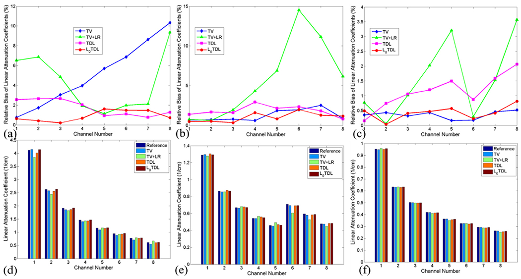
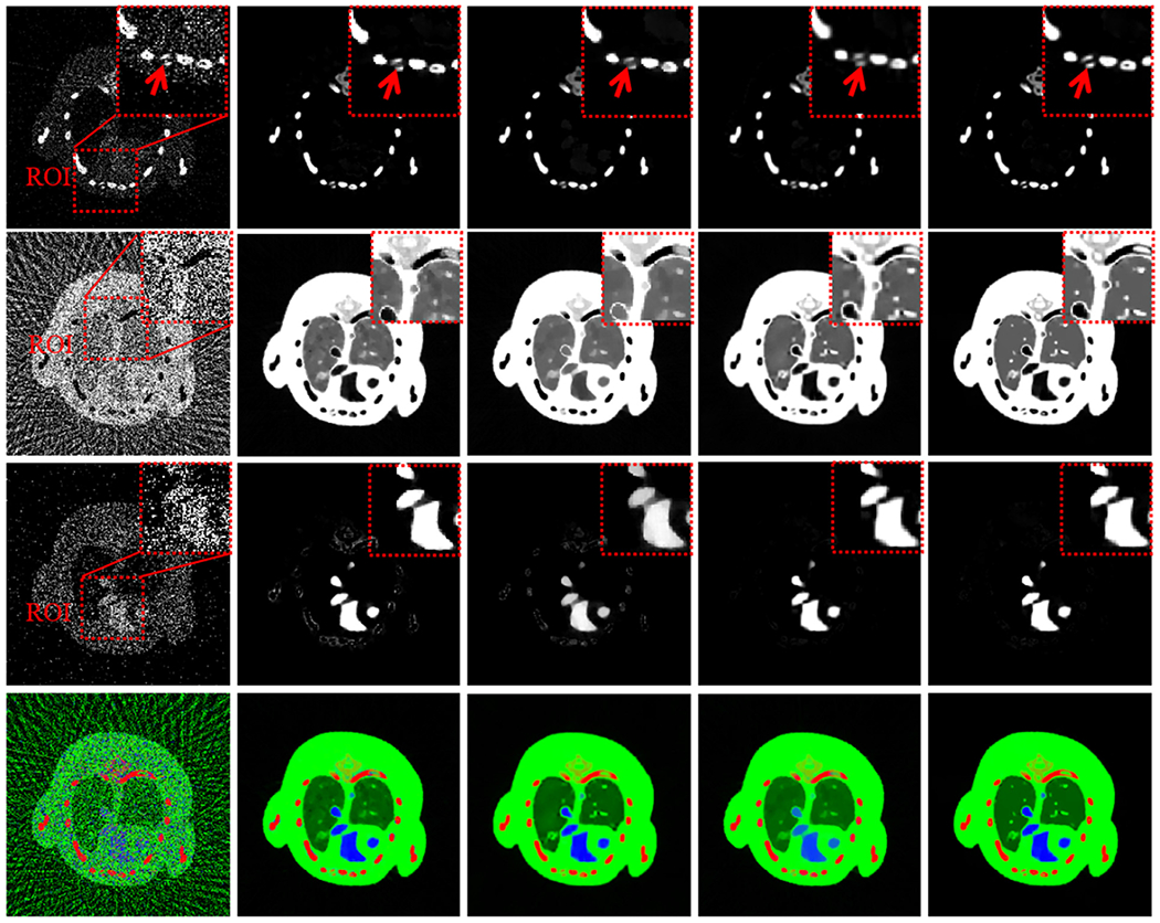
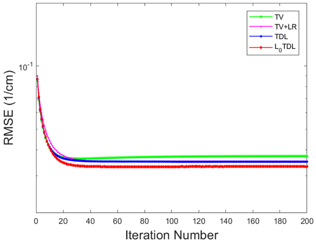
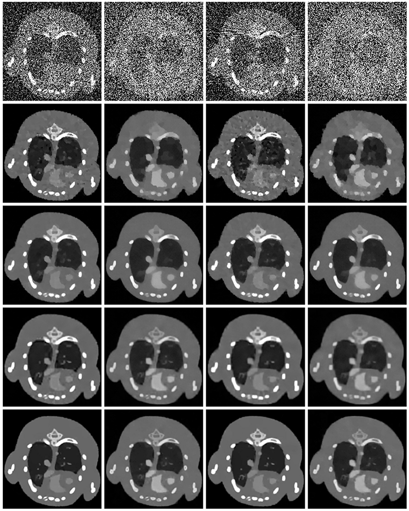
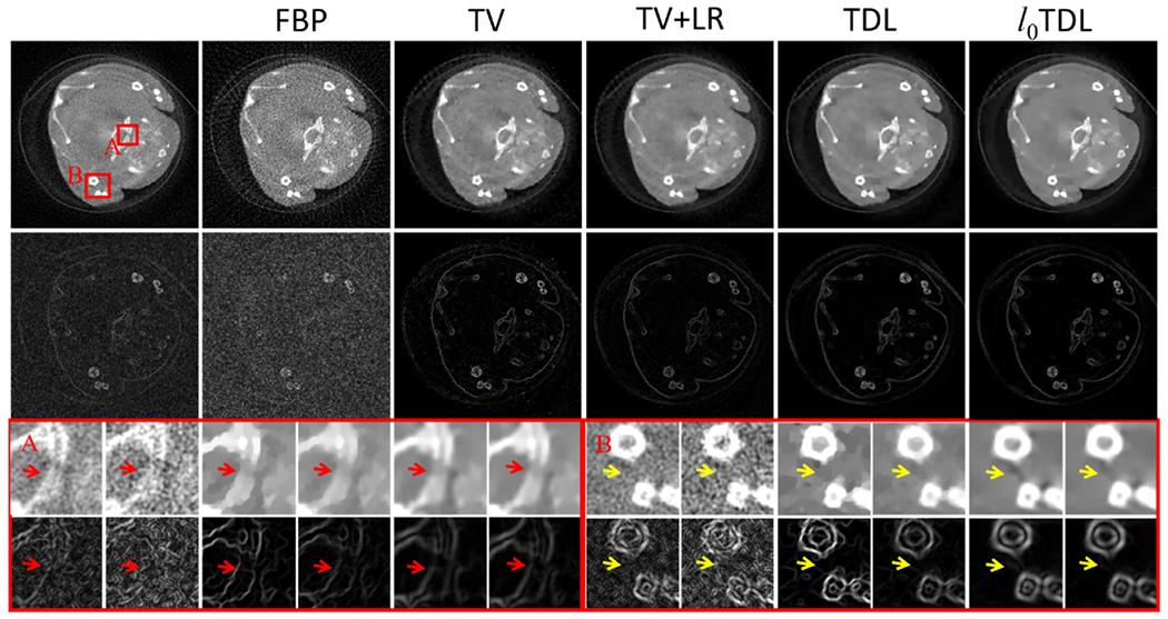
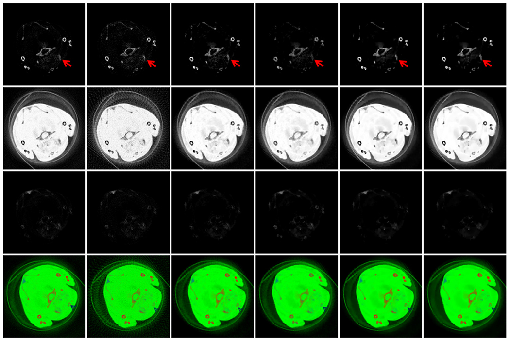
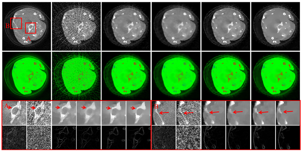
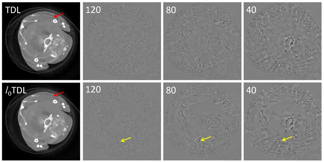
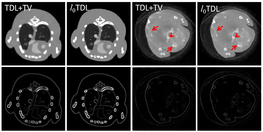
Spectral computed tomography (CT) has a great superiority in lesion detection, tissue characterization and material decomposition. To further extend its potential clinical applications, in this work, we propose an improved tensor dictionary learning method for low-dose spectral CT reconstruction with a constraint of image gradient ℓ ₀-norm, which is named as ℓ ₀TDL. The ℓ ₀TDL method inherits the advantages of tensor dictionary learning (TDL) by employing the similarity of spectral CT images. On the other hand, by introducing the ℓ ₀-norm constraint in gradient image domain, the proposed method emphasizes the spatial sparsity to overcome the weakness of TDL on preserving edge information. The split-bregman method is employed to solve the proposed method. Both numerical simulations and real mouse studies are perform to evaluate the proposed method. The results show that the proposed ℓ ₀TDL method outperforms other competing methods, such as total variation (TV) minimization, TV with low rank (TV+LR), and TDL methods.

Keywords: Image reconstruction; Low-dose; Sparse-view; Spectral computed tomography (CT); Tensor dictionary; ℓ0-norm of image gradient.

Fig. 1.

The flowchart of the ℓ₀TDL method.

Fig. 2.

Image quality assessments of the reconstructed images for the ℓ₀TDL method with respect to different σ.

Fig. 3.

Representative image slice of the mouse thorax phantom (channel 1) reconstructed by the ℓ₀TDL algorithm with different parameter settings. Each column represents different values of the same parameter and the rest parameters are fixed. The display window is [0 3] cm ⁻¹.

Fig. 4.

Same as Fig. 2 but for different η.

Fig. 5.

Same as Fig. 1 but for different ε.

Fig. 6.

Same as Fig. 2 but for different L.

Fig. 7.

Same as Fig. 2 but for different λ*.

Fig 8.

The mouse thorax phantom (left) and the corresponding gradient image (right).

Fig. 9.

Reconstruction results of the modified mouse thorax phantom. The first two rows are the reconstructed and gradient images from 160 projections and the last two rows are the magnified images of ROIs A and B. The display window of the reconstructed images is [0 3] cm⁻¹ and the gradient images are in [0 0.8] cm ⁻¹.

Fig. 10.

Same as Fig. 9 but from 106 projections.

Fig. 11.

Same as Fig. 9 but from 80 projections

Fig. 12.

Mean values and the corresponding relative biases for bone (1^st column), iodine contrast agent (2^nd column) and soft tissue (3^rd column).

Fig. 13.

Material decomposition results of images reconstructed by different algorithms from 80 projections. The 1^st to 3^rd rows are the decomposed bone, soft tissue and iodine contrast agent components, respectively. The 4th row is the true color images where red, green and blue regions represent the three basis materials. (For interpretation of the references to colour in this figure legend, the reader is referred to the web version of this article.)

Fig. 14.

The convergence curves in terms of average RMSE vs. iteration number.

Fig. 15.

Reconstructed images from low-dose projections. The 1st and 3rd columns are channel 1 images in a display window [0 3] cm⁻¹, and the 2nd and 4th columns are channel 8 images in a display window [0 0.8] cm⁻¹. The first two columns are reconstructed from datasets with 4 × 10³ photons, and the last two columns are reconstructed from datasets with 3 × 10³ photons. From the 1st to 5th rows, the images are reconstructed by the FBP, TV, TV+LR, TDL and the proposed ℓ₀TDL algorithms, respectively.

Fig. 16.

From the left to right columns, images are reconstructed for the 1^st, 4^th, 9^th and 13^th channels and the display window is [0, 0.8] cm⁻¹

Fig. 17.

Same as Fig. 9 but reconstructed from the 120 projections of realistic mouse dataset. The first column is the originally reconstructed image using the FBP algorithm from full projections. The display window of the reconstructed images is [0, 0.8] cm⁻¹ and the gradient images are in [0, 0.4] cm⁻¹.

Fig. 18.

The three basic material decomposition of Fig. 17. From the first to third rows present the decomposition of bone, soft tissue and GNP. The fourth row is the fusion color image, where the red, green and blue represent the bone, soft tissue and GNP respectively. (For interpretation of the references to colour in this figure legend, the reader is referred to the web version of this article.)

Fig. 19.

Same as the Fig. 17 but reconstructed from the 80 projections. The second row images are color images instead of gradient images.

Fig. 20.

Same as the Fig. 19 but reconstructed from 40 projections.

Fig. 21.

Reconstructed images and the corresponding difference images for 1st channel with respect to different views using the TDL and ℓ₀TDL methods. The display windows of the reconstructed images and difference images are [0, 0.8] cm⁻¹ and [−0.3, 0.3] cm⁻¹, respectively.

Fig. 22.

The first two columns represent the reconstructed and corresponding gradient images from the 4th channel of numerically simulated mouse dataset using the TDL and ℓ₀TDL methods. The display window of the reconstructed image is [0, 0.8] cm⁻¹. The last two columns are the same as the first two columns but from the 13th channel of the realistic dataset and the display window of gradient images is [0, 0.4] cm⁻¹.

References

1. Zhang H, Xi X, Yan B, Han Y, X-ray CT image reconstruction from few-views via total generalized p-variation minimization, Eng. Med. Biol. Soc (2015) 5618. - PubMed
1. Wu W, Yu H, Gong C, Liu F, Swinging multi-source industrial CT systems for aperiodic dynamic imaging, Opt. Express 25 (2017) 24215. - PubMed
1. Wu W, Yu H, Wang S, Liu F, BPF-type region-of-interest reconstruction for parallel translational computed tomography, J. X-Ray Sci. Technol 25 (2017) 487–504. - PubMed
1. Hall EJ, Lessons we have learned from our children: cancer risks from diagnostic radiology, Pediatr. Radiol 32 (2002) 700–706. - PubMed
1. Kim K, Ye JC, Worstell W, Ouyang J, Rakvongthai Y, Fakhri GE, Li Q, Sparse-view spectral CT reconstruction using spectral patch-based low-rank penalty, IEEE Trans. Med. Imaging 34 (2015) 748–760. - PubMed
LinkOut - more resources