

Published Erratum
doi: 10.1002/hipo.23249.
Erratum
- PMID: 32812312
- PMCID: PMC8097602
- DOI: 10.1002/hipo.23249
Item in Clipboard
Published Erratum
Erratum
Hippocampus.
2020 Aug.
No abstract available
Conflict of interest statement
The authors declare no conflict of interest.
The authors declare that they have no conflicts of interest.
The authors declare no potential conflict of interest.
The authors declare no potential conflict of interest.
The authors declare no potential conflict of interest.
Figures
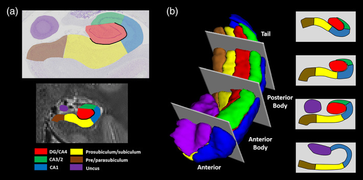
Subregions of the human hippocampus. (a) Top panel: a section of postmortem human hippocampus stained with cresyl violet to visualise cell bodies and overlaid with hippocampal subregion masks. Bottom panel: a T2‐weighted structural MRI scan of the human hippocampus overlaid with hippocampal subregion masks. (b) Left panel: a 3D model of hippocampal subregion masks with representative examples of demarcation points for anterior, anterior body, posterior body and tail portions of the subfields. Right panel: schematic representation of the subfields present in each portion of the hippocampus [Color figure can be viewed at wileyonlinelibrary.com ]
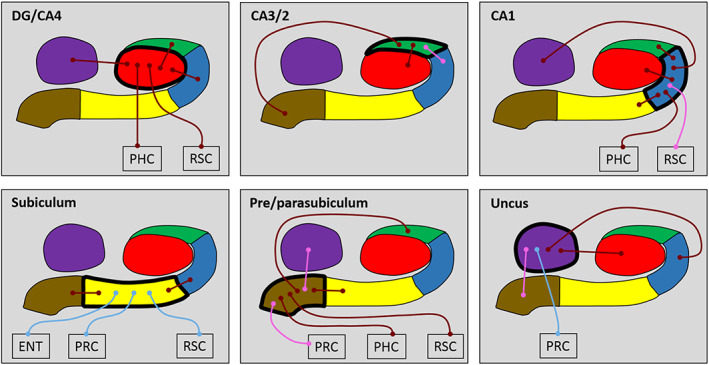
Results of the whole subfield analyses for the young and older participant groups. The relevant subfield in each panel is outlined in a thick black line. The thin lines with circular termini represent significant correlations of activity with the activity in other hippocampal subfields and/or extra‐hippocampal ROIs. Dark red lines represent significant correlations common to both young and old groups. Light blue lines represent significant correlations present only in the young group. Pink lines represent significant correlations present only in the older group. DG/CA4 (red), CA3/2 (green), CA1 (blue), subiculum (yellow), pre/parasubiculum (brown), uncus (purple); ENT, entorhinal cortex; PHC, posterior parahippocampal cortex; PRC, perirhinal cortex; RSC, retrosplenial cortex [Color figure can be viewed at wileyonlinelibrary.com ]
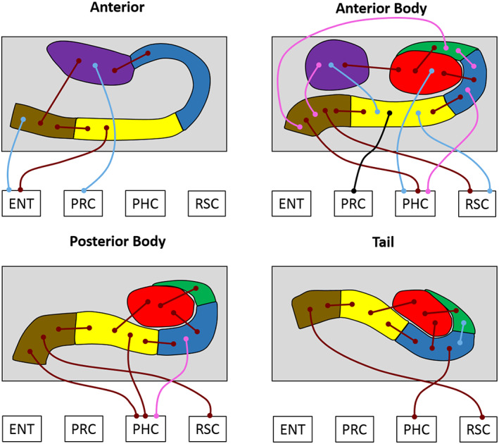
Results of the longitudinal subfield analyses for the young and older participant groups. The thin lines with circular termini represent significant correlations of activity with the activity in other hippocampal subfields and/or extra‐hippocampal ROIs. Dark red lines represent significant correlations common to both young and old groups. Light blue lines represent significant correlations present only in the young group. Pink lines represent significant correlations present only in the older group. The black line represents a significant increase in FC for young compared to older participants. DG/CA4 (red), CA3/2 (green), CA1 (blue), subiculum (yellow), pre/parasubiculum (brown), uncus (purple); ENT, entorhinal cortex; PHC, posterior parahippocampal cortex; PRC, perirhinal cortex; RSC, retrosplenial cortex [Color figure can be viewed at wileyonlinelibrary.com ]
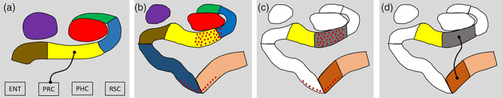
Exploratory analysis. (a) Results of the contrast of the young > older group for the AB hippocampus revealing the subiculum had reduced FC with the PRC in the older participants (thin black line with circular termini). DG/CA4 (red), CA3/2 (green), CA1 (blue), subiculum (yellow), pre/parasubiculum (brown), uncus (purple); ENT, entorhinal cortex; PHC, posterior parahippocampal cortex; PRC, perirhinal cortex; RSC, retrosplenial cortex. (b) Representation of our original segmentation scheme overlaid with red dots representing areas implicated in early (Stage 1) tau accumulation (adapted from Lace et al., 2009). Note the pattern of tau accumulation is largely restricted to the CA1‐subiculum transition region (predominantly within our subiculum mask) and the transentorhinal cortex (predominantly within our perirhinal cortex mask) during these early stages. (c) Representation of our amended segmentation scheme to create ROIs for the putatively tau‐affected CA1‐subiculum transition zone (grey) and transentorhinal cortex (rust). Amended ROIs for the medial subiculum (yellow) and lateral perirhinal cortex (coral) are also displayed. (d) Results for the contrast of the young > older group revealed the CA1‐subiculum transition region had reduced FC with the transentorhinal cortex in the older participants (thin black line with circular termini) [Color figure can be viewed at wileyonlinelibrary.com ]
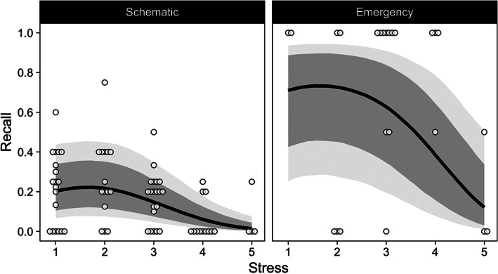
The relation between stress and recall for Schematic and Emergency questions. Points are proportions of recalled items for individual subjects at each level of stress (horizontal noise was added to display overlapping subjects). Lines are fitted recall probabilities (with 95% and 80% CIs as grey shades) from multilevel logistic regression model
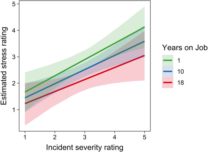
The relation between participants' stress ratings (y‐axis), the coder's rating of event severity rating (x‐axis) and years on job. Lines and shades indicate regression lines and 95% CIs, respectively, from multilevel regression model [Color figure can be viewed at wileyonlinelibrary.com ]

Photo of four happy neuroscientists taken in December 2017 at Lynn Nadel's Festschrift meeting. From left; Lynn Nadel, May‐Britt Moser, John O'Keefe, Richard Morris, far left: Neil Burgess. Photo taken by Tor Grønbech [Color figure can be viewed at wileyonlinelibrary.com ]
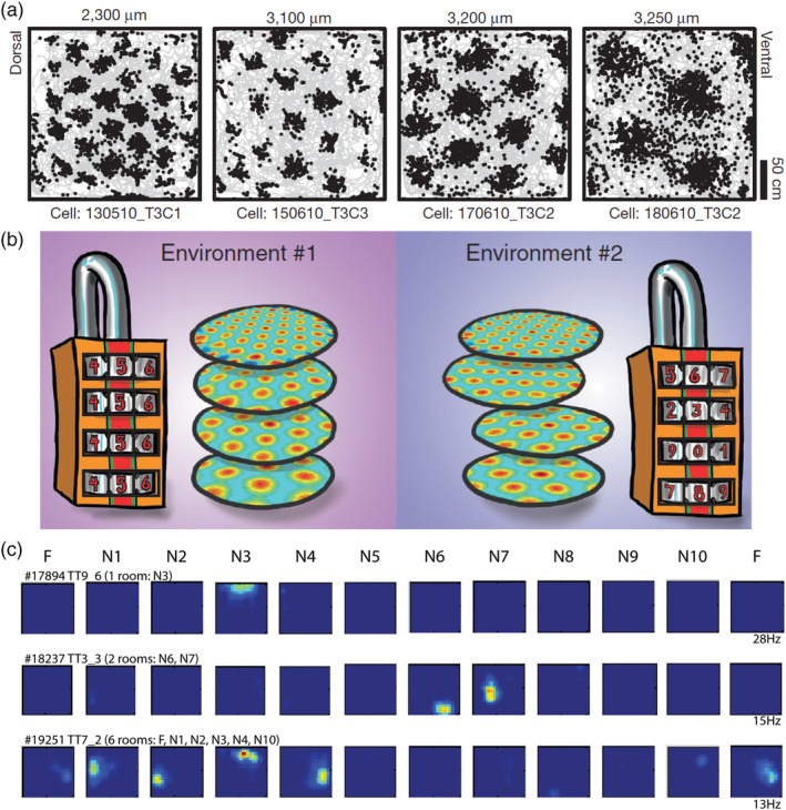
Unique place cell ensemble activity in hippocampus could be generated from multiple grid cell maps in medial entorhinal cortex. (a) Four example grids with distinct inter‐field spacing. Neuronal spikes (black dots) overlaid on the trajectory of the rat (grey). Dorsoventral location from the brain surface is indicated. Note the increasing inter‐field spacing at consecutively more ventrally recorded grid cells. Adapted from Stensola et al. (2012). (b) Suggested mechanism for the formation of unique place cell maps in hippocampus. In different environments, grid cells within one module shift and rotate together, whereas grid cells in different modules could shift and rotate independently. In this way, a small number of grid modules can encode a vast number of environments by the vast number of combinations of shifts and rotations, like the number combinations on a locker. Source: Drawing by Håkon Fyhn. Adapted from Rowland and Moser (2014). (c) Color‐coded rate maps from three example place cells showing distribution of firing rate between 11 environments (blue, no firing; red, peak firing). Each row comprises ratemaps from one neuron recorded in a familiar room (F, first and last column) and 10 novel rooms (N1–N10). Note that a population of place cells form unique ensemble activity in each room, with cells being active in one room and silent in another. If active, the position of the fields in two different rooms do not correlate, thus, an example of global remapping. Adapted from Alme et al. (2014) [Color figure can be viewed at wileyonlinelibrary.com ]
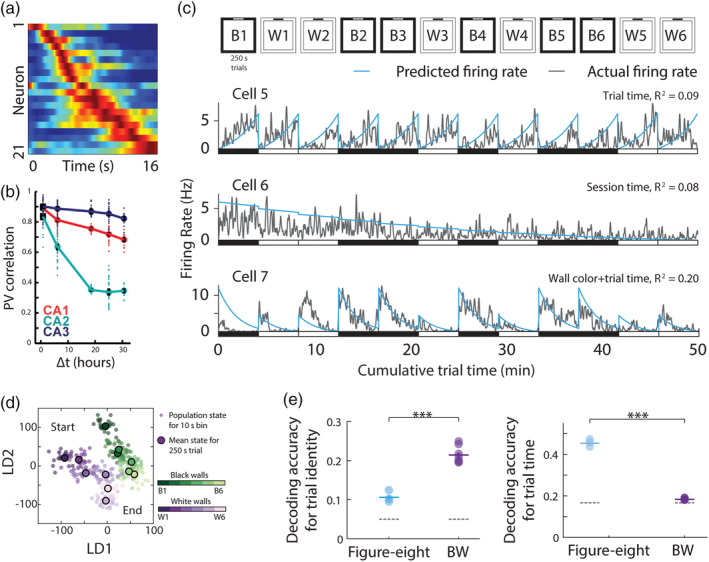
Time codes in hippocampus and entorhinal cortex. (a) Time cells in hippocampus tile a time interval within an episode when a rat runs on a treadmill. Each row represents the normalized firing rate of one neuron (blue, no firing; red, peak firing of that neuron) and the neurons are sorted by their peak firing time. Adapted from Kraus, Robinson, White, Eichenbaum, and Hasselmo (2013). (b) Stability of location specific activity of place cells in CA1 (red), CA2 (green), and CA3 (blue) was measured as population vector correlations between pairs of recordings. The black error bars report the mean ± SEM for pair‐wise comparisons at each time interval. Over time the population activity of CA2 (green) and CA1 neurons (red) decrease as a function of elapsed time between recording sessions. Adapted from Mankin, Diehl, Sparks, Leutgeb, and Leutgeb (2015). (c) Temporal codes in lateral entorhinal cortex. Top: experimental design; Animals ran 12 times 250 s trials in boxes with either black or white walls. Bottom: example general linear model fits for cells with selectivity for trial time (Cells 5 and 7) or session time (Cell 6), with the observed firing rate shown in grey, and predicted firing rate in blue, suggesting that the passage of time is encoded in firing rates of individual cells. (d) Two‐dimensional projections of neural population responses during the experiment depicted in “a”. Axes correspond to the first two linear discriminants (LD1 and LD2; arbitrary units). The wall color of each trial is indicated by a shade of green (black walls) or purple (white walls) with progression of shade from dark to light indicating the progression of trials. Population responses showed a progression corresponding to the temporal order of the experiment. (e) Left: comparison of decoding accuracy for trial identity when the rat is either engaged in alternating left/right laps on a figure eight maze or during the 12 black/white trials‐experiment (BW) depicted in “c”. Decoding accuracy for trial identity is higher during free foraging in BW than in the figure eight maze (p < .0001). Right: same as left, but for time epochs within a trial. Decoding of trial time is higher in the figure eight maze than in BW (p < 10−10). Grey‐dotted lines indicate chance levels. c–e adapted from (Tsao et al., 2018) [Color figure can be viewed at wileyonlinelibrary.com ]
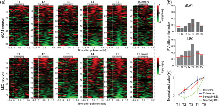
Olfactory coding in lateral entorhinal cortex (LEC) and hippocampus. Adapted from Igarashi et al. (2014). (a) Rats were trained to associate two odors with two different reward locations. Responses are shown for cells with significant activity at the cue port during training of naïve animals (T1) until reaching asymptotic performance (85% correct, T5). Right column contains error trials during T5. Each row shows data for one cell around the time of odor sampling (starting from white dashed line). Top: distal CA1 cells; bottom: LEC cells. Selectivity is color coded (−1 and + 1 indicate complete selectivity for banana [red] and chocolate [green], respectively). (b) Population odor selectivity was measured by correlating population activity obtained during sampling of the two different odors. Higher values indicate more odor‐selective population coding. Red lines indicate 95th percentiles from shuffled distributions. Odor selectivity develops in both LEC and hippocampus in parallel to improved performance. Odor selectivity decreases during error trials (T5e) compared to during a similar number of correct trials (T5d). (c) Development of task performance, gamma coherence and selectivity in CA1 and LEC. Variables are normalized onto a scale from 0 (T1) to 1 (T5) (mean ± SEM). Odor selectivity increases faster in LEC compared to CA1 [Color figure can be viewed at wileyonlinelibrary.com ]
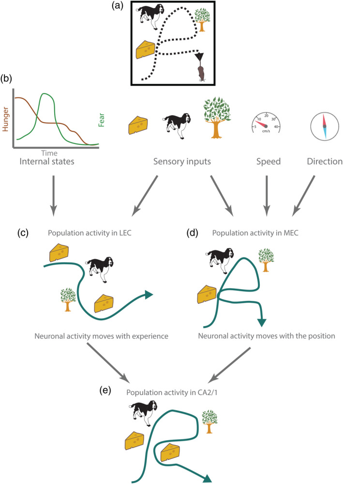
Schematic overview of spatial and temporal codes in entorhinal cortex and hippocampus. (a) Agent moves and have four experiences (two of them in the same position). Black dashed line indicates path of the animal. (b) Information concerning internal states of the animal, sensory inputs, and self‐motion signals reach entorhinal cortex. (c) Neuronal population activity (green line) in lateral entorhinal cortex moves with the experience of the agent. (d) Neuronal population activity (green line) in medial entorhinal cortex moves with the position of the animal. (e) Neuronal population activity (green line) in CA2 and CA1 in hippocampus moves with the position and experience of the animal. Episodes are mapped in a spatiotemporal framework conveyed from entorhinal cortex. Neural activity is more similar (but not identical) during two visits to the same location [Color figure can be viewed at wileyonlinelibrary.com ]
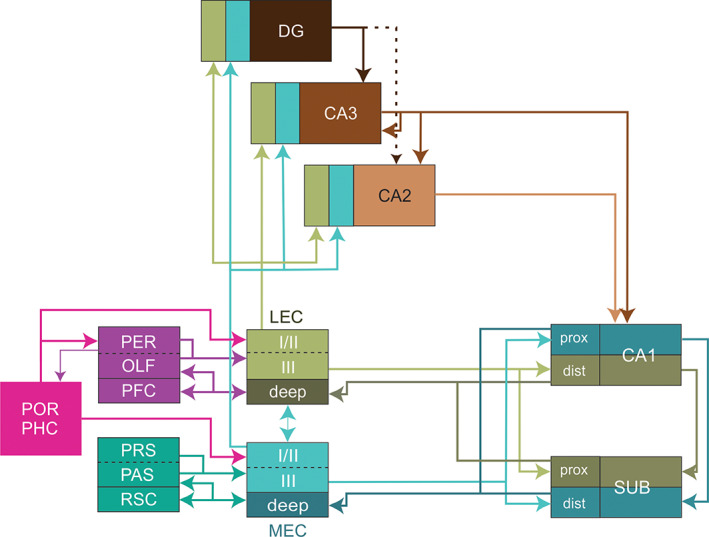
Schematic representation of the proposed updated version of the wiring scheme of the parahippocampal‐hippocampal system. The lateral and medial entorhinal cortex mediate parallel input streams, conveying integrated representations of two complementary sets of cortical inputs to the hippocampus. The lateral entorhinal cortex (LEC) receives strong inputs from perirhinal (PER), orbitofrontal, medial prefrontal and insular cortices (PFC), and olfactory structures (OLF) including the olfactory bulb and the olfactory or piriform cortex. In contrast, MEC receives main inputs from presubiculum (PRS), parasubiculum (PAS), and retrosplenial cortex (RSC). The postrhinal/parahippocampal cortex (POR/PHC) provides inputs to both MEC and LEC as well as to PER. Dashed dividers in boxes imply that incoming projections distribute to both components of the box. CA3, CA2, CA1, subfields of the hippocampus proper; DG, dentate gyrus; dist, distal part; prox, proximal part [Color figure can be viewed at wileyonlinelibrary.com ]
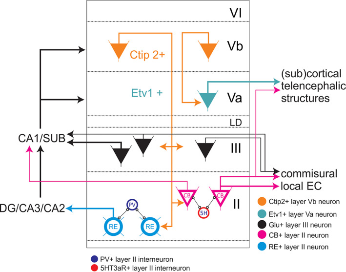
Summary of shared neuron types and local circuit motifs of the lateral and medial entorhinal cortex. Because very little to nothing is known concerning Layer VI, no neurons and circuits are indicated. In Layer II, we show the two types of principal neurons, reelin (RE) and calbindin (CB) positive, and their specific local connectivity to parvalbumin (PV) and 5HT3a‐receptor (5H) expressing interneurons, respectively. Also shown are the main projections to hippocampal fields and intrinsic and commissural projections. Not included is the observation that these two populations of principal cells do communicate through a separate class of pyramidal neurons. In Layer III, about 40% of the neurons projecting to CA1 and subiculum do give rise to commissural collaterals. Pyramidal cells in Layer III show a relatively strong developed local excitatory network (not indicated). In Layer V, we indicate that VB neurons project to Va as well as to Layers II and III. Note that although data indicate that the superficially projecting Layer Vb neurons also project to Laver Va, conclusive evidence for that is still lacking, so we have depicted as if these respective projections originate from different principal neurons. Inputs to layers and identified neurons therein are not indicated since they differ between LEC and MEC. CA3, CA2, CA1 subfields of the hippocampus proper; CB, calbindin‐positive neuron; DG, dentate gyrus; EC, entorhinal cortex; LD, lamina dissecans; RE, reelin‐positive neuron [Color figure can be viewed at wileyonlinelibrary.com ]
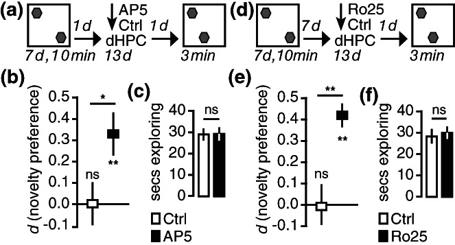
Blocking NMDAR activity in the dorsal hippocampus during the retention interval prevents the decay of long‐term object location memories. (a) During sampling, animals were exposed to two copies of a junk objects for 10 min a day for the seven consecutive days that remained at the same locations. This protocol leads to long‐term object location memories lasting for about 8 days (Migues et al., 2016). Twenty‐four hours after the last sampling session, animals were infused with AP5 or Veh into the dorsal hippocampus twice daily for 13−days. The following day, 14−days after the end of sampling, animals were returned to the open field for the probe trial, where one of the original objects was moved to a novel location. (b) Animals infused with AP5 preferred to explore the relocated object, thus expressing memory for the original object locations, while animals infused with vehicle explored both objects the same. (c) Both groups expressed the same overall exploratory activity during the probe trial. (d) Using the same behavioral protocol, animals were infused with Ro25‐6981 during the memory retention interval. (e) Only animals that received the GluN2B‐selective antagonist Ro25‐6981 preferred exploring the object at the novel location. (f) There were no differences in overall exploratory activity. *p−<−.05, **p−<−.01
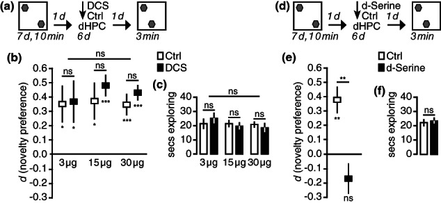
Enhancing NMDAR activity in the dorsal hippocampus with D‐Serine, but not D‐Cyloserine accelerates the natural forgetting of long‐term object location memories. (a) We used the same protocol as in Figure 14 with the difference that the retention interval was only 7 days. Animals were infused with the partial NMDAR agonist D‐Cycloserine during each day of this 6‐day memory retention interval. Animals were tested 7 days after the end of sampling, at a time when they naturally express long‐term object location memory in this paradigm (Migues et al., 2016). (b) At all doses tested, animals infused with D‐Cycloserine preferred to explore the object at the novel location, just like animals that had received Veh. Group differences were absent. (c) Overall exploratory activity during the probe trial was the same for all groups. (d) Instead of D‐Cycloserine, animals were infused with the NMDAR co‐agonist D‐Serine during the 6‐day memory retention interval. (e) Animals that had received D‐Serine showed no object location preference during the probe trial, while animals infused with Veh preferred to explore the moved object. (f) There were no differences in overall exploratory activity. *p−<−.05, **p−<−.01
Erratum for
-
Functional connectivity along the anterior-posterior axis of hippocampal subfields in the ageing human brain.Hippocampus. 2019 Nov;29(11):1049-1062. doi: 10.1002/hipo.23097. Epub 2019 May 6. Hippocampus. 2019. PMID: 31058404 Free PMC article.
-
NMDA receptor activity bidirectionally controls active decay of long-term spatial memory in the dorsal hippocampus.Hippocampus. 2019 Sep;29(9):883-888. doi: 10.1002/hipo.23096. Epub 2019 May 6. Hippocampus. 2019. PMID: 31058409
-
The puzzle of spontaneous alternation and inhibition of return: How they might fit together.Hippocampus. 2019 Aug;29(8):762-770. doi: 10.1002/hipo.23102. Epub 2019 Jun 3. Hippocampus. 2019. PMID: 31157942
-
Memory, stress, and the hippocampal hypothesis: Firefighters' recollections of the fireground.Hippocampus. 2019 Dec;29(12):1141-1149. doi: 10.1002/hipo.23128. Epub 2019 Jun 29. Hippocampus. 2019. PMID: 31254433
-
Episodic memory: Neuronal codes for what, where, and when.Hippocampus. 2019 Dec;29(12):1190-1205. doi: 10.1002/hipo.23132. Epub 2019 Jul 23. Hippocampus. 2019. PMID: 31334573 Review.
-
Neurons and networks in the entorhinal cortex: A reappraisal of the lateral and medial entorhinal subdivisions mediating parallel cortical pathways.Hippocampus. 2019 Dec;29(12):1238-1254. doi: 10.1002/hipo.23145. Epub 2019 Aug 13. Hippocampus. 2019. PMID: 31408260 Review.
Publication types
Grants and funding
LinkOut - more resources
Full Text Sources
